24 Graphs

24.1 Principles of Graphics

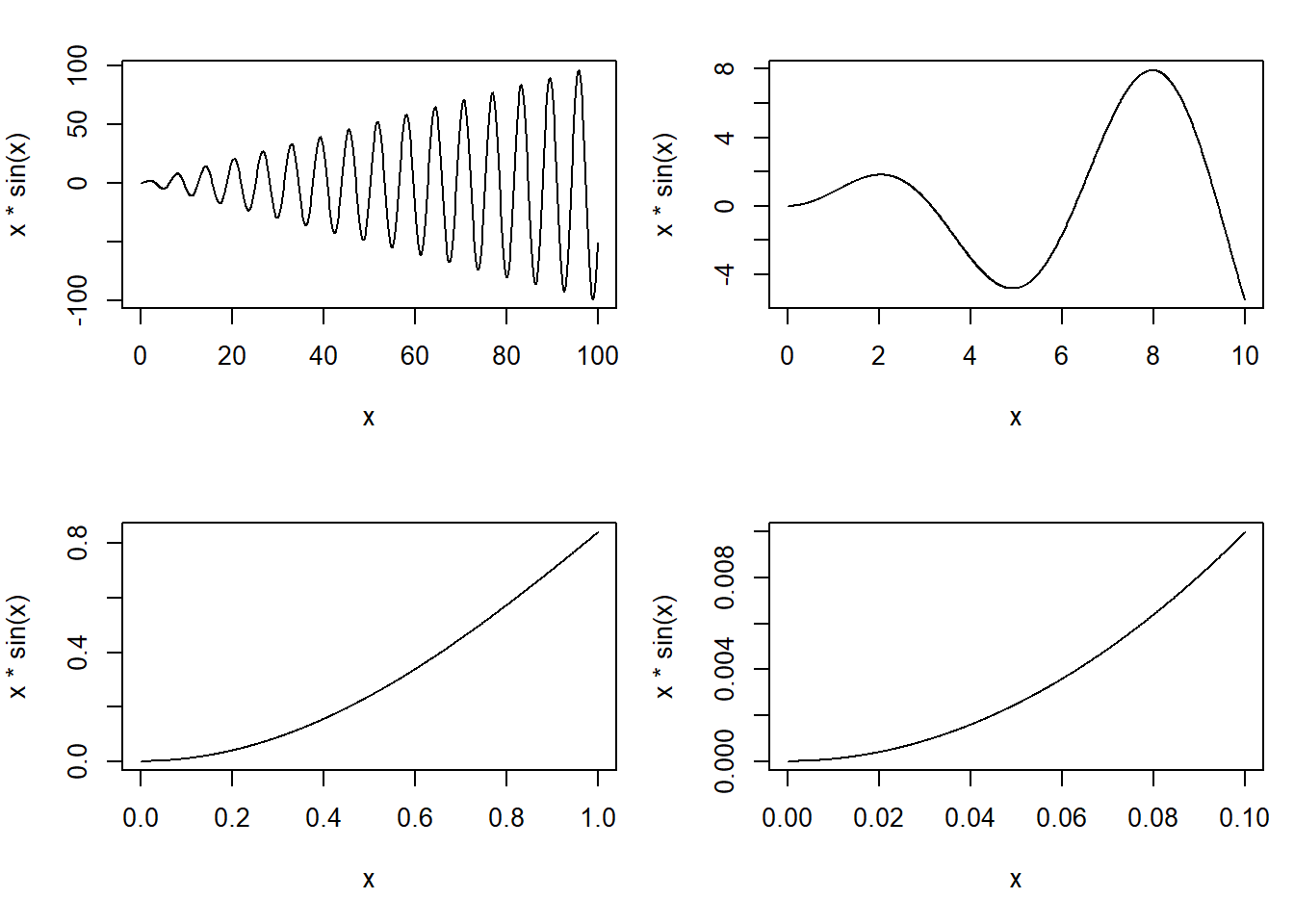
1. Show comparisons

You should always be comparing at least two things.

2. Show causality, mechanism, explanation, systematic structure

Generally, it’s difficult to prove that one thing causes another thing even with the most carefully collected data. But it’s still often useful for your data graphics to indicate what you are thinking about in terms of cause.

3. Show multivariate data

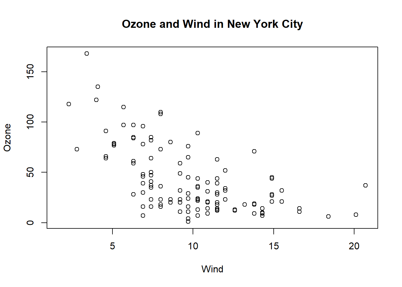
The point is that data graphics should attempt to show this information as much as possible, rather than reduce things down to one or two features that we can plot on a page… From the plot it seems that there is a slight negative relationship between the two variables….This example illustrates just one of many reasons why it can be useful to plot multivariate data and to show as many features as intelligently possible. In some cases, you may uncover unexpected relationships depending on how they are plotted or visualized.

4. Integrate evidence

Data graphics should make use of many modes of data presentation simultaneously, not just the ones that are familiar to you or that the software can handle. One should never let the tools available drive the analysis; one should integrate as much evidence as possible on to a graphic as possible.

5. Describe and document the evidence

Data graphics should be appropriately documented with labels, scales, and sources. A general rule for me is that a data graphic should tell a complete story all by itself. Is there enough information on that graphic for the person to get the story? While it is certainly possible to be too detailed, I tend to err on the side of more information rather than less.

6. Content, Content, Content

Analytical presentations ultimately stand or fall depending on the quality, relevance, and integrity of their content. This includes the question being asked and the evidence presented in favor of certain hypotheses. Starting with a good question, developing a sound approach, and only presenting information that is necessary for answering that question, is essential to every data graphic.

24.2 Types of Graphs

Visualizing the data via graphics can be important at the beginning stages of data analysis to understand basic properties of the data, to find simple patterns in data, and to suggest possible modeling strategies. In later stages of an analysis, graphics can be used to “debug” an analysis, if an unexpected (but not necessarily wrong) result occurs, or ultimately, to communicate your findings to others.

We will make a distinction between exploratory graphs and final graphs:

Exploratory graphs are usually made very quickly and a lot of them are made in the process of checking out the data, developing a personal understanding of the data and to prioritize tasks for follow up. Details like axis orientation or legends, while present, are generally cleaned up and prettified if the graph is going to be used for communication later.

24.2.1 One-dimension graphs

Graph	Code	Use
Five-number summary	`fivenum()`, `summary()`
Boxplots	`boxplot(pollution$pm25, col = "blue")`	Commonly plot outliers that go beyond the bulk of the data
Barplot	`table(pollution$region) %>% barplot(col = "wheat")`	For visualizing categorical data, with the number of entries for each category being proportional to the height of the bar
Histogram	`hist(pollution$pm25, col = "green", breaks = 100)` `rug(pollution$pm25)` `abline(v = 12, lwd = 2)` `abline(v = median(pollution$pm25), col = "magenta", lwd = 4)`	Check skewness of the data, symmetry, multi-modality, and other features
Density plot	`a <- density(airquality$Ozone, na.rm = TRUE)` `plot(a)`	Computes a non-parametric estimate of the distribution of a variables

24.2.2 Multi-dimension graphs

Graph	Code	Use
Multiple 1-D plots	`boxplot(pm25 ~ region, data = pollution, col = "red")` `par(mfrow = c(2, 1), mar = c(4, 4, 2, 1))` `hist(subset(pollution, region == "east")$pm25, col = "green")` `with(subset(airquality, Month == 5), points(Wind, Ozone, col = "blue"))` `hist(subset(pollution, region == "west")$pm25, col = "green")> boxplot(pm25 ~ region, data = pollution, col = "red")` `par(mfrow = c(2, 1), mar = c(4, 4, 2, 1))` `hist(subset(pollution, region == "east")$pm25, col = "green")` `with(subset(airquality, Month == 5), points(Wind, Ozone, col = "blue"))` `hist(subset(pollution, region == "west")$pm25, col = "green")`	For seeing the relationship between two variables, especially when one is naturally categorical
Scatterplots	`with(pollution, plot(latitude, pm25, col = region)) > abline(h = 12, lwd = 2, lty = 2)` `levels(pollution$region)` `par(mfrow = c(2, 1), mar = c(4, 4, 2, 1))` `hist(subset(pollution, region == "east")$pm25, col = "green")` `hist(subset(pollution, region == "west")$pm25, col = "green")`	Visualizing two continuous variables
Scatter plot matrix	`pairs(~var1+var2+var3+var4+var5, data=data, main="scatterplot matrix")`	It is used to find the correlation between a variable and other variables, and to select the important variables, which is also known as variable selection
Smooth scatterplots	`with(airquality, {plot(Temp, Ozone), lines(loess.smooth(Temp, Ozone))`	Similar to scatterplots but rather plots a 2-D histogram. Can be useful for scatterplots with many many data points

24.3 The Base Plotting System

The base plotting system is the original plotting system for R. The basic model is sometimes referred to as the “artist’s palette” model. The idea is you start with blank canvas and build up from there.

You will typically start with a plot function (or similar plot creating function) to initiate a plot and then annotate the plot. If you don’t have a completely well-formed idea of how you want your data to look, you’ll often start by “throwing some data on the page” and then slowly add more information to it as our thought process evolves.

There are a few downsides though:

You can’t go backwards once the plot has started.
While the base plotting system is nice in that it gives you the flexibility to specify these kinds of details to painstaking accuracy, sometimes it would be nice if the system could just figure it out for you.
It’s difficult to describe or translate a plot to others because there’s no clear graphical language or grammar that can be used to communicate what you’ve done.

24.3.1 How to Create a Base Plot?

First, you must read the data into R with read.csv(). For example, the avgpm25.csv dataset contains the annual mean PM2.5 averaged over the period 2008 through 2010
```
class <- c("numeric", "character", "factor", "numeric", "numeric")
pollution <- read.csv("data/avgpm25.csv", colClasses = class)  
```
Explicitly launch a graphics device.
Call a plotting function to make a plot (Note: if you are using a file device, no plot will appear on the screen).
Annotate the plot if necessary.
Explicitly close graphics device with dev.off() (this is very important!).

Example:

# Open PDF device; create 'myplot.pdf' in my working directory
pdf(file = "myplot.pdf", width = 4, height = 3) # The height and width arguments are in units of inches.
# Create plot and send to a file (no plot appears on screen) 
with(faithful, plot(eruptions, waiting))
# Annotate plot; still nothing on screen 
title(main = "Old Faithful Geyser data") 
# Close the PDF file device 
dev.off() 
# Now you can view the file 'myplot.pdf' on your computer

Let’s further detail each of the steps involved in creating a base plot.

24.3.2 Graphics Devices

We can think of a graphics device as being a platform upon which the plot is created. If we create a plot, then a default graphics device is automatically opened for the plot to appear upon. In other words, when you make a plot in R, it has to be “sent” to a specific graphics device.

The most common place for a plot to be “sent” is the screen device. Functions like plot() in base, xyplot() in lattice, or qplot in ggplot2 will default to sending a plot to the screen device. Therefore, when making a plot, you need to consider how the plot will be used to determine what device the plot should be sent to.

The list of devices supported by your installation of R is found in ?Devices.

Using the commands pdf, postscript, jpeg, png, or bmp, we can also produce graphics in the formats that correspond to these names.
The jpeg, png, and bmp graphics are all raster-style graphics, which may translate poorly when included in a document.
In contrast, the pdf, postscript, and windows metafile (win.metafile, available on Windows) formats allow for vector-style graphics, which are scaleable, and better suited to integration in documents.

Vector	Bitmap
Good for line drawings and plots with solid colors using a modest number of points	good for plots with a large number of points, natural scenes or web-based plots
pdf (line-type graphics, resizes well, usually portable)	png (good for line drawings or images with solid colors)
svg (XML-based scalable vector graphics; supports animation and interactivity)	jpeg (good for plotting many many many points, does not resize well)
win.metafile	tiff
postscript	bmp

It is possible to open multiple graphics devices (screen, file, or both), for example when viewing multiple plots at once. Plotting can only occur on one graphics device at a time, though.

One way of having more than one plot visible is to open additional graphics devices. In a Windows environment this is done by using the command windows() before each additional plot.

To create a graphics device without a plot, we call the function that is specific to our operating system (that is, windows for Windows, quartz for Mac, and X11 for Unix).

The currently active graphics device can be found by calling dev.cur()

Every open graphics device is assigned an integer starting with 2 (there is no graphics device 1). You can change the active graphics device with dev.set(<integer>).

24.3.3 Graphics Parameters

Graphics parameters control how output appears on graphics devices. To get a complete list with their current values, type par(). Some of the parameters mentioned above, namely pch, lwd and col, are examples of graphics parameters. To get the value of a specific parameter, for example pch, type par("pch").

Some graphics parameters can apply to one or more plots, and others only make sense when applied to graphics devices. For example, to change the symbol for a single plot, we could include the argument pch = 2 in the call to the plot function. However, we could also make this change for all graphics that are produced on the device.

To change a graphics parameter for the graphics device, we use the par command. These are some examples:

par(mfrow = c(a,b)) where a and b are integers, will create a matrix of plots on one page, with a rows and b columns. These will be filled by rows; use mfcol if you wish to fill them by columns.

Example:

par(mfrow = c(2, 2), mar=c(5, 4, 2, 1))
curve(x*sin(x), from = 0, to = 100, n = 1001)
curve(x*sin(x), from = 0, to = 10, n = 1001)
curve(x*sin(x), from = 0, to = 1, n = 1001)
curve(x*sin(x), from = 0, to = 0.1, n = 1001)

par(mar = c(bottom, left, top, right)) will create space around each plot, in which to write axis labels and titles. Measurements are in units of character widths.
par(oma = c(bottom, left, top, right)) will create space around the matrix of plots (an outer margin). Measurements are in units of character widths.
par(las = 1) rotates labels on the y-axis to be horizontal rather than vertical.
par(pty = "s") forces the plot shape to be square. The alternative is that the plot shape is mutable, which is the default, and corresponds to pty ="m".

24.3.4 Make a Plot with `plot(x,y)`

plot(x, y) is used to plot one vector against another, with the x values on the x-axis and the y values on the y-axis.

The plot command offers a wide variety of options for customizing the graphic. Each of the following arguments can be used within the plot statement, singly or together, separated by commas

type = "p": Determines the type of plot, with options:
- “p” for points (the default);
- “l” for lines;
- “b” for both, with gaps in the lines for the points; …
Example:
```
with(airquality, plot(Wind, Ozone, 
    main = "Ozone and Wind in New York City",
    type = "p")
)
```
points(x, y): To add points (x[1], y[1]), (x[2], y[2]), … to the current plot.
lines(x, y): To add lines.
abline(v = xpos) and abline(h = ypos): to draw vertical or horizontal lines. - col: Both points and lines take the optional input from col (e.g. “red”, “blue”, etc.). The complete list of available colours can be obtained by the colours function (or colors).

Example: # Plot with a Regression Line
- First make the plot (as above).
- Fit a simple linear regression model using the lm() function.
- Take the output of lm() and pass it to the abline() function which automatically takes the information from the model object and calculates the corresponding regression line
text(x, y, labels): To add the text labels [i] at the point (x[i], y[i]). The optional input pos is used to indicate where to position the labels in relation to the points.
title(text): To add a title, where text is a character string.
main = "Plot title goes in here": provides the plot title.
xlab = " " / ylab = " ": To add axis labels.

Note: In a call to plot, the arguments for main, sub, and xlab and ylab can be character strings or expressions that contain a mathematical expression. For mathematical typesetting you can use the functions expression(require graphics) and bquote(base):

Example:
```
...
xlab = expression(alpha),
ylab = expression(100 %*% (alpha^3 - alpha^2) + 15),
# Mix of mathematical expressions and character strings into a single expression by using the paste function
main = expression(paste("Function: ",
   f(alpha) == 100 %*% (alpha^3 - alpha^2) + 15)),
...
```
xlab = expression(alpha) tells R to interpret alpha in the context of the MML (mathematical markup language), producing an α as the label for the x-axis.
pch = k: Determines the shape of points, with k taking a value from 1 to 25.
lwd = 1: line width, default 1.
xlim = c(a,b)/ `ylim = c(a,b): Will set the lower and upper limits of the x-axis/y-axis to be a and b, respectively.

As an example we plot part of the parabola y² = 4x, as well as its focus and directrix. We make use of the surprisingly useful input type = "n", which results in the graph dimensions being established, and the axes being drawn, but nothing else.

Example:

x <- seq(0, 5, by = 0.01)
y.upper <- 2*sqrt(x)
y.lower <- -2*sqrt(x)
y.max <- max(y.upper)
y.min <- min(y.lower)
plot(c(-2, 5), c(y.min, y.max), type = "n", xlab = "x", ylab = "y")
lines(x, y.upper)
lines(x, y.lower)
abline(v=-1)
points(1, 0)
text(1, 0, "focus (1, 0)", pos=4)
text(-1, y.min, "directrix x = -1", pos = 4)
title("The parabola y^2 = 4*x")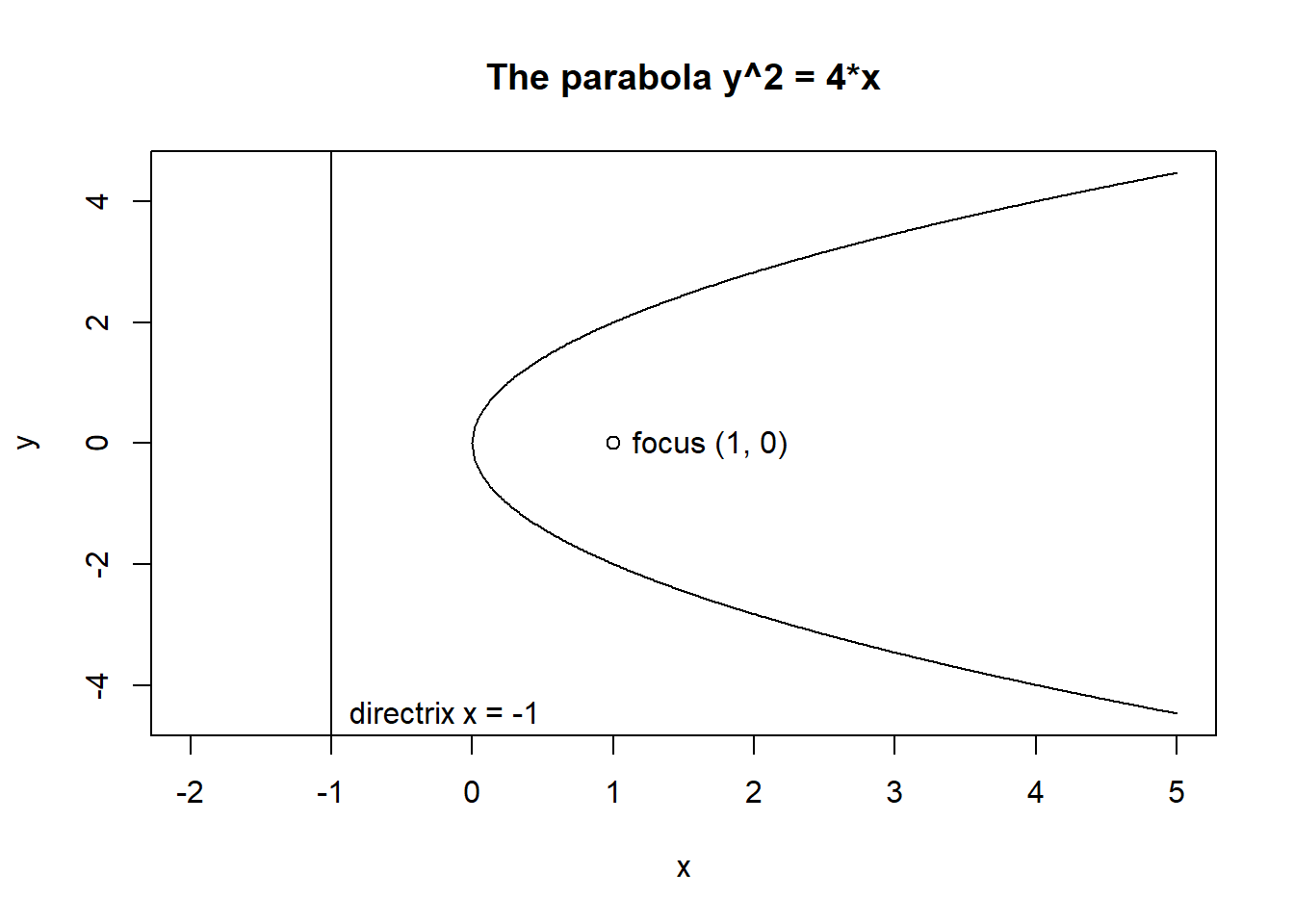

24.3.5 Augmenting a Plot

A traditional plot can be augmented using any of a number of different tools after its creation. A number of these different steps are detailed below:

Start by creating the plot object, which sets up the dimensions of the space, but omit any plot objects for the moment:

Example:

opar1 <- par(las = 1, mar=c(4,4,3,2))   
plot(ufc$dbh.cm, ufc$height.m, axes=FALSE, 
    xlab="",
    ylab="",
    type="n"
)

Next, we add the points. Here we use different colours and symbols for different heights of trees: those that are realistic, and those that are not, which may reflect measurement errors. We use the vectorised ifelse() function:

Example:
```
points(ufc$dbh.cm, ufc$height.m,     
  col = ifelse(ufc$height.m > 4.9, "darkseagreen4", "red"),
  pch = ifelse(ufc$height.m > 4.9, 1, 3)
)
```
Then we add axes. The following are the simplest possible calls. We can also control the locations of the tickmarks, and their labels; we can overlay different axes, change colour, and so on. ?axis provides the details:

Example:
```
axis(1)
axis(2)
```
We can next add axis labels using margin text (switching back to vertical direction for the y-axis text):

Example:
```
opar2 <- par(las=0)
mtext("Diameter (cm)", side=1, line=3)
mtext("Height (m)", side=2, line=3)
```
Wrap the plot in the traditional frame. As before, we can opt to use different line types and different colours:

Example:
```
box()
```
Finally, we add a legend:

Example:
```
legend(x = 60, y = 15, c("Normal trees", "A weird tree"),
    col=c("darkseagreen3", "red"),
    pch=c(1, 3),
    bty="n"
)
```
Note the first two arguments: the location of the legend can also be expressed relative to the graph components, for example, by “bottomright”.
If we wish, we can return the graphics environment to a previous state:
```
par(opar1)
```

Check out the playwith package, which provides interaction with graphical objects at a level unattainable in base R.

24.3.6 Color in Plots

Typically we add color to a plot, not to improve its artistic value, but to add another dimension to the visualization. It makes sense that the range and palette of colors you use will depend on the kind of data you are plotting. Careful choices of plotting color can have an impact on how people interpret your data and draw conclusions from them.

The function colors() lists the names of (657) colors you can use in any plotting function. Typically, you would specify the color in a (base) plotting function via the col argument.

The grDevices package has two functions, they differ only in the type of object that they return:

colorRamp: Take a palette of colors and return a function that takes values between 0 and 1.
```
pal <- colorRamp(c("red", "blue")) 
pal(0)
```
The numbers in the matrix will range from 0 to 255 and indicate the quantities of red, green, and blue (RGB) in columns 1, 2, and 3 respectively. there are over 16 million colors that can be expressed in this way.

The idea here is that you do not have to provide just two colors in your initial color palette; you can start with multiple colors and colorRamp() will interpolate between all of them.
colorRampPalette: Takes a palette of colors and returns a function that takes integer arguments and returns a vector of colors interpolating the palette (like heat.colors() or topo.colors()).
```
pal <- colorRampPalette(c("red", "yellow"))
pal(3)
```
Returns 3 colors in between red and yellow. Note that the colors are represented as hexadecimal strings.
Note that the rgb() function can be used to produce any color via red, green, blue proportions and return a hexadecimal representation:
```
rgb(0, 0, 234, maxColorValue = 255)
```
Part of the art of creating good color schemes in data graphics is to start with an appropriate color palette that you can then interpolate with a function like colorRamp() or colorRampPalette().

For improved color palettes you can use the RColorBrewer package. Here is a display of all the color palettes available from this package:

library(RColorBrewer) 
display.brewer.all()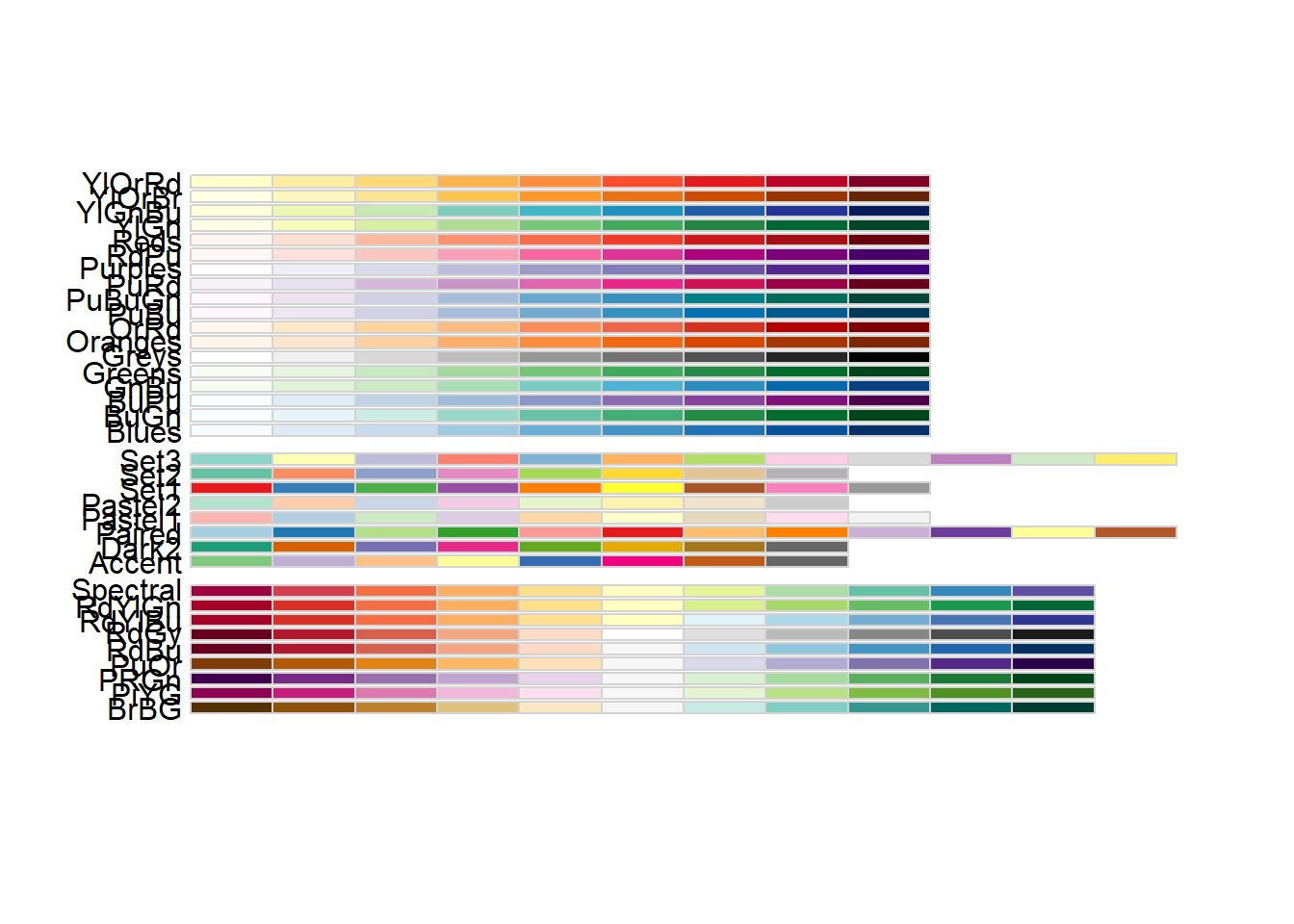

The brewer.pal() function creates nice looking color palettes especially for thematic maps:
```
library(RColorBrewer)
(cols <- brewer.pal(3, "BuGn"))
```
```
[1] "#E5F5F9" "#99D8C9" "#2CA25F"
```
These three colors make up your initial palette. Then you can pass them to colorRampPalette() to create my interpolating function.
```
pal <- colorRampPalette(cols)
```
Now you can plot your data using this newly created color (ramp) palette:
```
image(volcano, col = pal(20))
```
The smoothScatter() function is very useful for making scatterplots of very large datasets:
```
set.seed(1)
x <- rnorm(10000)
y <- rnorm(10000) 
smoothScatter(x, y)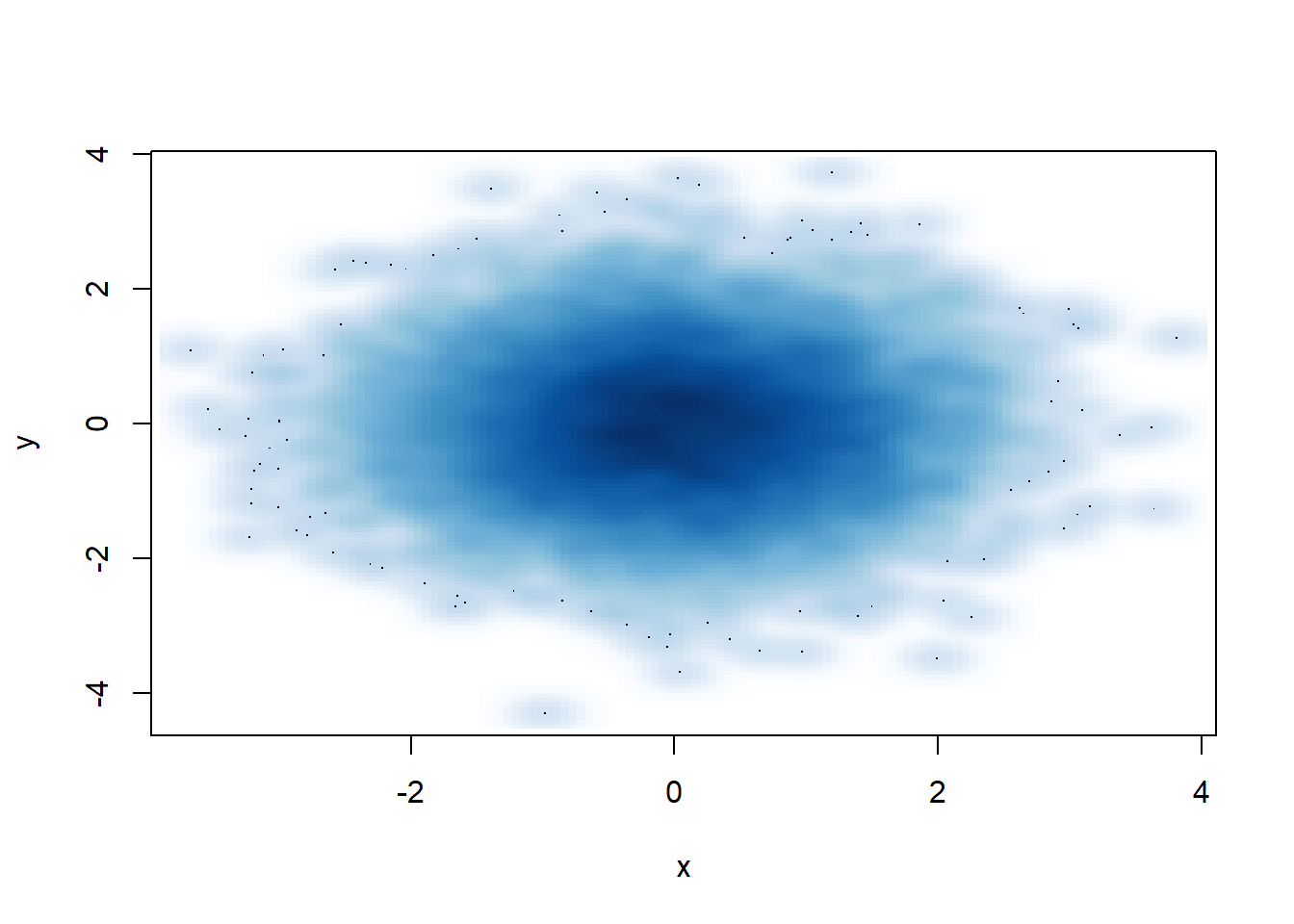
```
Adding transparency: Color transparency can be added via the alpha parameter to rgb() to produce color specifications with varying levels of transparency.
```
rgb(1, 0, 0, 0.1)
```
```
[1] "#FF00001A"
```
Transparency can be useful when you have plots with a high density of points or lines. If you add some transparency to the black circles, you can get a better sense of the varying density of the points in the plot.
```
# x, y from the previous example
plot(x, y, pch = 19, col = rgb(0, 0, 0, 0.15))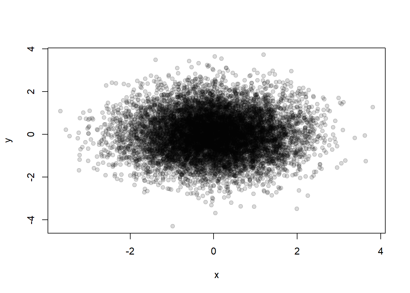 
```

24.3.7 Copying Plots

Note that copying a plot is not an exact operation, so the result may not be identical to the original:

## Copy my plot to a PNG file  (follows the previous code from pdf creation)
dev.copy(png, file = "geyserplot.png") 

## Don't forget to close the PNG device! 
dev.off()

24.3.8 Complementary Packages

graphics: contains plotting functions for the “base” graphing systems, including plot, hist, boxplot and many others
grdevices: contains all the code implementing the various graphics devices, including X11, PDF, PostScript, PNG, etc.

24.4 The Lattice System

Trellis graphics are a data visualisation framework developed at the Bell Labs, which have been implemented in R as the lattice package.

Trellis graphics are a set of techniques for displaying multidimensional data. They allow great flexibility for producing conditioning plots; that is, plots obtained by conditioning on the value of one of the variables.

To use Trellis graphics you must first you must load the lattice package with the library function: library(lattice).

24.4.1 When to Use Trellis Plots

Lattice plots tend to be most useful for conditioning types of plots, i.e. looking at how y changes with x across levels of z. These types of plots are useful for looking at multidimensional data and often allow you to squeeze a lot of information into a single window or page.
With the lattice system, plots are created with a single function call, such as xyplot() or bwplot().
Note that there is no real distinction between the functions that create or initiate plots and the functions that annotate plots because it all happens at once.
Another difference from base plotting is that things like margins and spacing are set automatically. This is possible because entire plot is specified at once via a single function call.
The notion of panels comes up a lot with lattice plots because you typically have many panels in a lattice plot (each panel typically represents a condition, like “region”).
Once a plot is created, you cannot “add” to the plot (but of course you can just make it again with modifications).

24.4.2 How to Use Lattice

To illustrate the use of the lattice package we use the ufc dataset, where dbh (diameter at breast height) and height vary by species. That is, the plots are conditioned on the value of the variable species.

Example:

# These plots display a distribution of values taken on by the variable dbh, divided up according to the value of the variable species
densityplot(~ dbh.cm | species, data = ufc) # A density plot
bwplot(~ dbh.cm | species, data = ufc) # # A box and whiskers plot
histogram(~ dbh.cm | species, data = ufc) # A histogram
# We plot height as a function of dbh.
xyplot(height.m ~ dbh.cm | species, data = ufc) # A scatterplot

All four commands require a formula object, which is described using ~and |.

If a dataframe is passed to the function, using the argument data, then the column names of the dataframe can be used for describing the model.
We interpret y ~ x | a as saying we want y as a function of x, divided up by the different levels of a.
If `a is not a factor then a factor will be created by coercion.
If we are just interested in x we still include the ~ symbol, so that R knows that we are specifying a model.
If we wish to provide within-panel conditioning on a second variable, then we use the group argument.

In order to display numerous lattice objects on a graphics device, we call the print function with the split and more arguments.

Example:

# Place a lattice object (called my.lat) in the top-right corner of a 3-row, 2-column graphics device, and allow for more objects
print(my.lat, split = c(2,1,2,3), more = TRUE)

See ?print.trellis for further details.

Graphics produced by lattice are highly customisable.

Example:

xyplot(height.m ~ dbh.cm | species,
    data = ufc,
    subset = species %in% list("WC", "GF"),
    panel = function(x, y, ...) {
        panel.xyplot(x, y, ...),       
        panel.abline(lm(y~x), ...)
    },
    xlab = "Diameter (cm)",
    ylab = "Height (m)"
    )

Note that the subset argument is a logical expression or a vector of integers, and is used to restrict the data that are plotted. We can also change the order of the panels using the index.cond argument (see ?xyplot for more details). The panels are plotted bottom left to top right by default, or top left to bottom right if the argument as.table = TRUE is supplied.

The panel argument accepts a function, the purpose of which is to control the appearance of the plot in each panel. The panel function should have one input argument for each variable in the model, not including the conditioning variable.

24.5 3D Plots

R provides considerable functionality for constructing 3D graphics, using either the base graphics engine or the lattice package. However, its is recommended to use the lattice package, because the data can be supplied to the lattice functions in a familiar structure: observations in rows and variables in columns, unlike that required by the base 3D graphics engine (observations in a grid).

Example:

ufc.plots <- read.csv("../data/ufc-plots.csv")
str(ufc.plots)
library(lattice)
wireframe(vol.m3.ha ~ east * north,
    main = expression(paste("Volume (", m^3, ha^{-1}, ")", sep =        "")),
    xlab = "East (m)", ylab = "North (m)",
    data = ufc.plots
    )

To learn more about base-graphics 3D plots, run the demonstrations demo(persp) and demo(image) and look at the examples presented.

24.6 ggplot2

ggplot2 is one of the most elegant and most versatile systems for making graphs. ggplot2 implements the grammar of graphics, a coherent system for describing and building graphs.

ggplot2 splits the difference between base and lattice in a number of ways. Taking cues from lattice, the ggplot2 system automatically deals with spacings, text, titles but also allows you to annotate by “adding” to a plot.

You can find more information in the Graphs section here.

24.6.1 Installation

install.packages("ggplot2")
library(ggplot2)

A typical plot with the ggplot package looks as follows:

data(mpg)
qplot(displ, hwy, data = mpg)

In ggplot2, aesthetics are the things we can see (e.g. position, color, fill, shape, line type, size). You can use aesthetics in ggplot2 via the aes() function:

ggplot(data, aes(x=var1, y=var2))

24.6.2 Geometric objects

Geometric objects are the plots or graphs you want to put in the chart.

You can use geom_point() to create a scatterplot, geom_line() to create a line plot, and geom_boxplot() to create a boxplot in the chart.

help.search("geom_", package="ggplot2")

In ggplot2, geom is also the layers of the chart. You can add in one geom object after another, just like adding one layer after another layer.

ggplot(data, aes(x=var1, y=var2)) + 
  geom_point(aes(color="red"))

24.6.3 Plotly

Plotly JS allows you to create interactive, publication-quality charts. You can create a Plotly chart using ggplot:

install.packages("plotly")
set.seed(12)
var1 <- rnorm(100, mean=1, sd=1)
var2 <- rnorm(100, mean=2, sd=1)
data <- data.frame(var1, var2)
gg <- ggplot(data) + geom_line(aes(x=var1, y=var2))
g <- ggplotly(gg)

24.1 Principles of Graphics

24.2 Types of Graphs

24.2.1 One-dimension graphs

24.2.2 Multi-dimension graphs

24.3 The Base Plotting System

24.3.1 How to Create a Base Plot?

24.3.2 Graphics Devices

24.3.3 Graphics Parameters

24.3.4 Make a Plot with plot(x,y)

24.3.5 Augmenting a Plot

24.3.6 Color in Plots

24.3.7 Copying Plots

24.3.8 Complementary Packages

24.4 The Lattice System

24.4.1 When to Use Trellis Plots

24.4.2 How to Use Lattice

24.5 3D Plots

24.6 ggplot2

24.6.1 Installation

24.6.2 Geometric objects

24.6.3 Plotly

24.3.4 Make a Plot with `plot(x,y)`