alpha_df <- data.frame(index = seq(from = 1, to = 15, by = 1),
                       power = seq(from = 14, to = 0, by = -1))
alpha_df$alpha_0.01 <- 0.01 * (1 - 0.01) ^ alpha_df$power
alpha_df$alpha_0.2 <- 0.2 * (1 - 0.2) ^ alpha_df$power
alpha_df$alpha_0.4 <- 0.4 * (1 - 0.4) ^ alpha_df$power
alpha_df$alpha_0.6 <- 0.6 * (1 - 0.6) ^ alpha_df$power
alpha_df$alpha_0.8 <- 0.8 * (1 - 0.8) ^ alpha_df$power
alpha_df$alpha_1 <- 1 * (1 - 1) ^ alpha_df$power39 Forecasting with Exponential Smoothing
The exponential smoothing functions are one of the most popular forecasting approaches among the traditional time series forecasting models. This approach, conceptually, is close to the \(MA\) approach, as both are based on forecasting the future values of the series by averaging the past observations of the series.
The \(SES\) model shares some of the attributes of the \(WMA\) model, as both models forecast the future values of the series by a weighted average of the past observations of the series. The main distinction between the two is that the SES model is utilizing all the previous observations, whereas the WMA model is using only the most recent \(m\) observations (for a model with a rolling window of a length of \(m\)).
In both the \(MA\) and \(SES\), the user must specify a single parameter: in \(MA\), the window width (\(w\)); and in exponential smoothing, the smoothing constant (\(\alpha\)). In both cases, the parameter determines the importance of fresh information over older information. In fact, the two smoothers are approximately equal if the window width of the moving average is equal to \(w = 2/ \alpha − 1\).
Like the moving average, simple exponential smoothing should only be used for forecasting series that have no trend or seasonality.
39.1 Simple Exponential Smoothing Model
The simple exponential smoothing (SES) is the simplest forecasting model among the exponential smoothing family. The main assumption of this model is that the series stays at the same level (that is, the local mean of the series is constant) over time, and therefore, this model is suitable for series with neither trend nor seasonal components.
The main attribute of the \(SES\) model is the weighted average technique, which is based on the exponential decay of the observation weights according to their chronological distance (i.e., series index or timestamp) from the first forecasted values. The decay rate of the observation weights is set by \(\alpha\), a constant between 0 and 1 called the smoothing constant.
We can write the exponential smoother equation as a weighted average of all past observations, with exponentially decaying weights:
\[F_{t+1} = F_t + \alpha \epsilon_t\] where \(\epsilon_t\) is the forecast error (distance from the actual value) at time \(t\) and \(F_t\) is the previous forecast (Ft). If the forecast was too high in the last period, the next period is adjusted down. The amount of correction depends on the value of the smoothing constant \(\alpha\).
The smoothing constant \(\alpha\), which is set by the user, determines the rate of learning. A value close to \(1\) indicates fast learning (that is, only the most recent values influence the forecasts), whereas a value close to \(0\) indicates slow learning (past observations have a large influence on forecasts). Hence, the choice of \(\alpha\) depends on the required amount of smoothing, and on how relevant the history is for generating forecasts. Default values that have been shown to work well are in the range \(0.1-0.2\). Trial and error can also help in the choice of \(\alpha\).
Example:
The following example demonstrates the decay of the weights of the observations on the most recent 15 observations, for values between 0.01 to 1:
Let’s plot the results:
library(plotly)
plot_ly(data = alpha_df) %>%
  add_lines(x = ~ index, y = ~ alpha_0.01, name = "alpha = 0.01") %>%
  add_lines(x = ~ index, y = ~ alpha_0.2, name = "alpha = 0.2") %>%
  add_lines(x = ~ index, y = ~ alpha_0.4, name = "alpha = 0.4") %>%
  add_lines(x = ~ index, y = ~ alpha_0.6, name = "alpha = 0.6") %>%
  add_lines(x = ~ index, y = ~ alpha_0.8, name = "alpha = 0.8") %>%
  add_lines(x = ~ index, y = ~ alpha_1, name = "alpha = 1") %>%
  layout(title = "Decay Rate of the SES Weights",
         xaxis = list(title = "Index"),
         yaxis = list(title = "Weight"))
39.1.1 Forecasting with the ses function
The forecast package provides a customized \(SES\) model with the ses function. The main arguments of this function are as follows:
initial: Defines the method for initializing the value of \(\hat Y_1\) , which can be calculated by using the first few observations of the series by setting the argument to simple, or by estimating it withetsmodel (an advanced version of the Holt-Winters model from the forecast package) when setting it to optimal.alpha: Defines the value of the smoothing parameter of the model. If set toNULL, the function will estimate it.h: Sets the forecast horizon.
Let’s use the ses function to forecast the monthly prices of the Robusta coffee data again. We will leave the last 12 months of the series as a testing set for benchmarking the model’s performance. We will do this using the ts_split function from the TSstudio package:
Example:
 The Coffee_Prices series is a mts object with 2 variables and 701 observations
 Frequency: 12
 Start time: 1960 1
 End time: 2018 5
library (TSstudio)
robusta_par <- ts_split(robusta, sample.out = 12)
train <- robusta_par$train
test <- robusta_par$testAfter we set the training and testing partition, we will use the training partition to train a \(SES\) model with the ses function:
library(forecast)
fc_ses <- ses(train, h = 12, initial = "optimal")
# Review the model details
fc_ses$model
Simple exponential smoothing
Call:
ses(y = train, h = 12, initial = "optimal")
Smoothing parameters:
alpha = 0.9999
Initial states:
l = 0.6957
sigma: 0.161
AIC AICc BIC
1989.646 1989.681 2003.252 We can review the model’s performance by using the test_forecast function:
Example:
test_forecast(actual = robusta,
              forecast.obj = fc_ses,
              test = test) %>%
  layout(title = "Robusta Coffee Prices Forecast vs. Actual",
         xaxis = list(range = c(2010, max(time(robusta)))),
         yaxis = list(range = c(1, 3)))
As we can see from the preceding forecast plot, the ses function is utilizing the training set to identify the series level by estimating the alpha parameter and the initial level of the model (or \(\hat Y_i\)). The forecast value level is fairly close to the value of the last observation of the series since the value, in this case, is close to \(1\). Since the goal of the \(SE\) model is to forecast the level of the series, the model won’t capture any short-term oscillation.
In the case of a flat forecast, the confidence intervals of the model play a critical role, since the level of uncertainty is higher. Therefore, it will be useful to evaluate whether the forecast values are within the model confidence interval bounds. We will use the plot_forecast function from the TSstudio package to create an interactive plot for the fs_ses model we created and plot the testing set:
plot_forecast(fc_ses) %>%
  add_lines(x = time(test) + deltat(test),
            y = as.numeric(test),
            name = "Testing Partition") %>%
  layout(title = "Robusta Coffee Prices Forecast vs. Actual",
         xaxis = list(range = c(2010, max(time(robusta)) +
                                  deltat(robusta))),
         yaxis = list(range = c(0, 4)))
As you can see from the preceding forecast plot, the testing set is within the range of the 80% confidence interval.
39.1.2 Model optimization with grid search
The ses function optimizes the values of the model parameters (\(\alpha\) and \(l_0\)) that minimize the sum of squared errors (SSE) of the model on the training set. An alternative optimization approach is to use a grid search.
A grid search is a powerful approach that’s used to identify the values of the model’s parameters that minimize the model error. In the case of the \(SES\) model, we will apply a grid search to identify the optimal value of that minimizes some error metric of the model (for example, MAPE, RMSE, and so on).
In the following example, we will use a grid search to tune the model parameters \(\alpha\) and \(l_0\), which minimize the model’s MAPE for the Robusta prices series. As we saw in the preceding performance plot of the Robusta forecast, there is a gap between the structure of the fitted values (marked in red) and the forecasted value (marked in green) since the \(SES\) model has a flat forecast. Therefore, we will split the model into training, testing, and validation partitions, and for each value of \(\alpha\), we will apply the following steps:
Train the \(SES\) model using the training partition and forecast the observations of the testing partition.
Evaluate the performance of the model on both the training and testing partition.
Append the training and testing partitions (in chronological order) and retrain the model on the new partition (training and testing) before forecasting the values of the validation partition.
Evaluate the performance of the second model on the validation partition.
Example:
# Set the training, testing, and validation partitions
robusta_par1 <- ts_split(robusta, sample.out = 24)
train1 <- robusta_par1$train
test1 <- ts_split(robusta_par1$test, sample.out = 12)$train
robusta_par2 <- ts_split(robusta, sample.out = 12)
train2 <- robusta_par2$train
valid <- robusta_par2$test
We will now use the train1 and test1 variables for training and testing partition, and train2 for retraining the model and validating the results on the valid partition. The following \(\alpha\) variable defines the search range. We will assign a sequence of values between \(0\) and \(1\) with an increment of \(0.01\) using the seq function:
Example:
alpha <- seq(from = 0, to = 1, by = 0.01)Since the value of alpha must be greater than zero, we will replace \(0\) with a small number that’s fairly close to zero:
alpha[1] <- 0.001We will use the lapply function to iterate on the model using the different values of \(\alpha\):
library(dplyr)
ses_grid <- lapply(alpha, function(i){
  md1 <- md_accuracy1 <- md2 <- md_accuracy2 <- results <- NULL
  md1 <- ses(train1, h = 12, alpha = i, initial = "simple")
  md_accuracy1 <- accuracy(md1, test1)
  md2 <- ses(train2, h = 12, alpha = i, initial = "simple")
  md_accuracy2 <- accuracy(md2, valid)
  resutls <- data.frame(alpha = i,
                        train = md_accuracy1[9],
                        test = md_accuracy1[10],
                        valid = md_accuracy2[10])
  }) %>%
  bind_rows()
As you can see in the following testing results, while \(\alpha = 1\) minimizes the MAPE on the training partition, \(\alpha=0.03\) minimizes the error rate on the testing partition. The results on the validation partition are following the same pattern as the testing partition, with an MAPE score of 9.98% on the testing partition and 6.60% on the validation partition:
plot_ly(data = ses_grid, x = ~ alpha, y = ~ train,
        line = list(color = 'rgb(205, 12, 24)'),
        type = "scatter",
        mode = "lines",
        name = "Training") %>%
  add_lines(x = ~ alpha, y = ~ test, line = list(color = "rgb(22, 96,
                                                   167)", dash = "dash"),
              name= "Testing") %>%
  add_lines(x = ~ alpha, y = ~ valid, line = list(color = "green", dash = "dot"), name = "Validation") %>%
  layout(title = "SES Model Grid Search Results",
         yaxis = list(title = "MAPE (%)"))
39.2 Holt method
The Holt method, also known as the double exponential smoothing model, is an expanded version of the \(SES\) model. It’s based on estimating the most recent level and trend with the use of two smoothing parameters, \(\alpha\) and \(\beta\). Once the model estimates the most recent level and trend (\(L_t\), and \(T_t\), respectively), it utilizes them to construct the series forecast using the following equation:
For a series with additive trend, \(\hat{Y}_{T+h} = L_T + hT_T\).
For a series with multiplicative trend, \(\hat{Y}_{T+1} = L_T \times hT_T\).
The forecast package provides an implementation of the Holt model with the holt function. This function automatically initializes the values of \(\hat L_1\) and \(\hat T_1\), and identifies the values of \(\alpha\) and \(\beta\) that minimize the \(SSE\) of the model on the training set.
In the following example, we will retrieve the US Gross Domestic Product (GDP) quarterly data from the Federal Reserve Economic Data (FRED) API using the Quandl package:
Example:
gdp <- fredr(
  series_id = "GDP",
  observation_start = as.Date("2010-01-01"),
  observation_end = as.Date("2019-01-01")
  )
head(gdp)
# A tibble: 6 × 5
date series_id value realtime_start realtime_end
<date> <chr> <dbl> <date> <date>
1 2010-01-01 GDP 14765. 2024-10-07 2024-10-07
2 2010-04-01 GDP 14980. 2024-10-07 2024-10-07
3 2010-07-01 GDP 15142. 2024-10-07 2024-10-07
4 2010-10-01 GDP 15309. 2024-10-07 2024-10-07
5 2011-01-01 GDP 15351. 2024-10-07 2024-10-07
6 2011-04-01 GDP 15558. 2024-10-07 2024-10-07 # Convert df to ts
gdp_ts <- ts(data = gdp$value,
start = c(2010, 1),
frequency = 4
)
str(gdp_ts) Time-Series [1:37] from 2010 to 2019: 14765 14980 15142 15309 15351 ...ts_info(gdp_ts) The gdp_ts series is a ts object with 1 variable and 37 observations
Frequency: 4
Start time: 2010 1
End time: 2019 1 You will notice in the following plot that the GDP series has a strong linear trend and no seasonal component (since the series is seasonally adjusted):
ts_plot(gdp_ts,
        title = "US Gross Domestic Product",
        Ytitle = "Billions of Dollars",
        Xtitle = "Source: U.S. Bureau of Economic Analysis /fred.stlouisfed.org")
Like we did previously, we will leave the last eight quarters for testing and train the model with the rest of the observations of the series with the holt function:
gdp_par <- ts_split(gdp_ts, sample.out = 8)
train <- gdp_par$train
test <- gdp_par$test
fc_holt <- holt(train, h = 8, initial = "optimal")
# Review the model's parameters
fc_holt$model
Holt's method
Call:
holt(y = train, h = 8, initial = "optimal")
Smoothing parameters:
alpha = 0.6836
beta = 1e-04
Initial states:
l = 14642.6449
b = 159.7415
sigma: 76.3941
AIC AICc BIC
354.8299 357.4386 361.6664 The initialized values of \(\hat L_1\) and \(\hat T_1\) of the function are relatively close to the values of the first observation of the series (\(Y_1 = 14642.64\)) and the average difference between each quarter. In addition, the selected \(\alpha\) of \(0.68\) indicated that the model heavily weighed the last observation of the series, \(Y_t\). On the other hand, the value of \(\beta\) is fairly close to zero, which indicates that updating the trend value from period to period doesn’t take into account the change in the level and carries the initial value of the trend, \(\hat{T_1}\), forward.
Let’s compare the model’s performance in the training and testing partitions with the accuracy function:
accuracy(fc_holt, test) ME RMSE MAE MPE MAPE MASE
Training set -0.4552329 70.93013 55.42122 -0.006041138 0.3248532 0.08781452
Test set 378.4198543 430.06268 378.41985 1.832552431 1.8325524 0.59960352
ACF1 Theil's U
Training set 0.04955818 NA
Test set 0.63394683 1.810023As you can see from the output of the accuracy function, the ratio between the error rate on the testing and training set is more than 6 times for the RMSE and 5.5 for the MAPE. This large ratio in the error metrics is mainly derived from the following two reasons:
The fitted values of the model on the training set are not bound by a linear line (as opposed to the forecast output).
The growth of the trend in the last few quarters shift from a linear rate of growth to an exponential rate.
The changes in the trend growth and the forecast can be observed with the test_forecast function:
test_forecast(gdp_ts, forecast.obj = fc_holt, test = test)While the Holt model was designed to handle time series with the linear trend, the exponential argument of the holt function provides the option to handle series with exponential or decaying trends when set to TRUE.
# Use the exponential argument to modify the growth pattern of the trend
# We seek a higher weight for the trend and we will set $\beta$ to 0.75
fc_holt_exp <- holt(train,
                    h = 8,
                    beta = 0.75,
                    initial = "optimal",
                    exponential = TRUE)
The output of this model is as follows:
fc_holt_exp$modelHolt's method with exponential trend
Call:
holt(y = train, h = 8, initial = "optimal", exponential = TRUE,
beta = 0.75)
Smoothing parameters:
alpha = 0.75
beta = 0.75
Initial states:
l = 14644.6809
b = 1.0113
sigma: 0.006
AIC AICc BIC
369.7359 371.4026 375.2051 We can review the model’s accuracy on the training and testing set with the accuracy function:
accuracy(fc_holt_exp, test) ME RMSE MAE MPE MAPE MASE
Training set -0.6785595 95.90897 79.45979 -0.00608536 0.4676049 0.1259035
Test set 158.0928706 194.12178 169.47521 0.76460898 0.8231642 0.2685322
ACF1 Theil's U
Training set -0.2405994 NA
Test set 0.5932521 0.8186658Similarly, we can plot the fitted and forecasted values against the actual data with the test_forecast functions:
test_forecast(gdp_ts, forecast.obj = fc_holt_exp, test = test)As you can see, the error rate of the second Holt model is more balanced, where the ration between the error on the testing and training set is \(2\) and \(2.1\) for the RMSE and MAPE metrics, respectively.
39.3 Holt-Winters model
The Holt-Winters model is the most advanced model among the exponential smoothing family of forecasting models. The Holt-Winters (HW) model is an extended version of the Holt model and can handle time series data with both trend and seasonal components. Forecasting the seasonal component requires a third smoother parameter and equation, in addition to the ones of the level and trend.
Both of the trend and seasonal components could have either an additive or multiplicative structure, which adds some complexity to the model as there are multiple possible combinations:
Additive trend and seasonal components.
Additive trend and multiplicative seasonal components.
Multiplicative trend and additive seasonal components.
Multiplicative trend and seasonal component.
The most common implementation of the HW model in R is the HoltWinters and hw functions from the stats and forecast packages. The main difference between the two functions is that the hw function can handle time series with an exponential or damped trend (similar to the Holt model).
In the following example, we will use the HoltWinters function to forecast the last 12 months of the USgas series.
Example:
# Diagnose the structure of the trend and seasonal components
data(USgas)
decompose(USgas) %>% plot()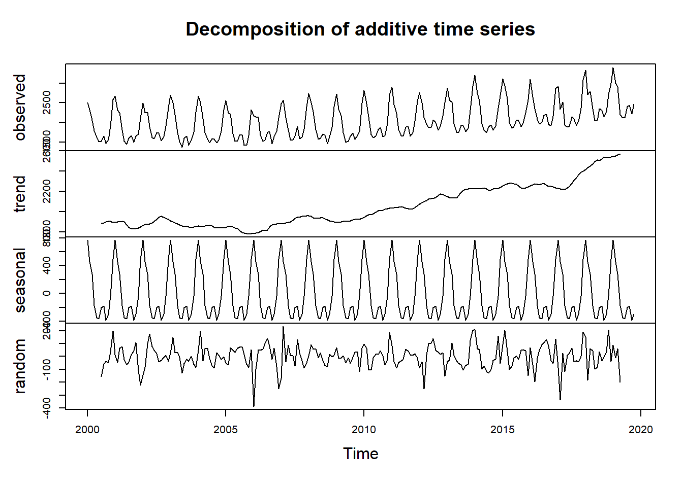
We can observe from the preceding plot that both the trend and seasonal components of the series have an additive structure. Like we did previously, we will create training and testing partitions using the last 12 months of the series to evaluate the performance of the model:
USgas_par <- ts_split(USgas, 12)
train <- USgas_par$train
test <- USgas_par$test
Next, we will use the HoltWinters model to forecast the last 12 months of the series (or the testing set):
md_hw <- HoltWinters(train)
# Review the parameters of the trained model
md_hw
Holt-Winters exponential smoothing with trend and additive seasonal component.
Call:
HoltWinters(x = train)
Smoothing parameters:
alpha: 0.371213
beta : 0
gamma: 0.4422456
Coefficients:
[,1]
a 2491.9930104
b -0.1287005
s1 32.0972651
s2 597.1088003
s3 834.9628439
s4 353.8593860
s5 318.1927058
s6 -173.0721496
s7 -346.6229990
s8 -329.7169608
s9 -112.1664217
s10 -140.3186476
s11 -324.5343787
s12 -243.9334551You will notice from the preceding model output that the model is mainly learning from the level and seasonal update (with \(\alpha = 0.37\) and \(\gamma = 0.44\) ). On the other hand, there is no learning from the trend initialized value \(\beta = 0\).
The next step is to forecast the next 12 months (or the values of the testing set) and evaluate the model’s performance with the accuracy and test_forecast functions:
fc_hw <- forecast(md_hw, h = 12)
accuracy(fc_hw, test)
ME RMSE MAE MPE MAPE MASE
Training set 7.828361 115.2062 87.67420 0.2991952 4.248131 0.7614222
Test set 51.013877 115.1555 98.06531 1.7994297 3.766099 0.8516656
ACF1 Theil's U
Training set 0.21911103 NA
Test set -0.01991923 0.3652142The accuracy metrics of the model are fairly balanced, with an \(MAPE\) of 4.2% in the training set and 3.8% in the testing set.
In the plot of the following model performance, you will notice that most of the forecast errors are related to the seasonal peak and the last observations of the series, which the model was underestimating:
test_forecast(actual = USgas,
              forecast.obj = fc_hw,
              test = test)
Plotting the fitted and forecasted values provides us with a better understanding of the model’s performance. As we can see in the preceding plot, the HW model is doing a good job of capturing both the series seasonal patterns. On the other hand, the model is missing the peak of the year during the month of January in most cases.
Note that alternatively, the model can be trained with a grid search in a similar manner to what we did with the \(SES\) model. In this case, there are three parameters to optimize: \(\alpha\), \(\beta\), and \(\gamma\). The TSstudio package provides a customized grid search function based on the backtesting approach for training a HoltWinters function.