30  Random Numbers

Simulation is an important (and big) topic for both statistics and for a variety of other areas where there is a need to introduce randomness.

Sometimes you want to implement a statistical procedure that requires random number generation or sample (i.e. Markov chain Monte Carlo, the bootstrap, random forests, bagging), or you want to simulate a system, then random number generators can be used to model random inputs.

Some example functions of random numbers probability distributions in R are these:

rnorm(n, mean = 0, sd = 1) ## generate random Normal variates with a given mean and standard deviation
dnorm(x, mean = 0, sd = 1, log = FALSE) ## evaluate the Normal probability density (with a given mean/SD) at a point (or vector of points)
pnorm(q, mean = 0, sd = 1, lower.tail = TRUE, log.p = FALSE)  ## evaluate the cumulative distribution function for a Normal distribution
qnorm(p, mean = 0, sd = 1, lower.tail = TRUE, log.p = FALSE) ## generate random Poisson variates with a given rate

Maybe the most common probability distribution to work with is the normal distribution (also known as the Gaussian).

Example:

x <- rnorm(10, 20, 2) 
summary(x)

   Min. 1st Qu.  Median    Mean 3rd Qu.    Max. 
  14.84   18.57   19.84   19.53   20.61   22.73 

30.1 Always Remember to Set Your Seed!

When simulating any random numbers it is essential to set the random number seed. Setting the random number seed with set.seed() ensures reproducibility of the sequence of random numbers.

Example:

set.seed(1)
rnorm(5)

[1] -0.6264538  0.1836433 -0.8356286  1.5952808  0.3295078

Example: Simulating a Linear Model

Suppose we want to simulate from the following linear model \(y=β_0+β_1x+ε\) where \(ε ∼ N(0, 22)\)

Assume \(x ∼ N(0, 12)\), \(β_0 = 0.5\) and \(β_1 = 2\). The variable x might represent an important predictor of the outcome y.

Here’s how you could do that in R:

## Always set your seed! 
set.seed(20) 
## Simulate predictor variable 
x <- rnorm(100) 
## Simulate the error term 
e <- rnorm(100, 0, 2) 
## Compute the outcome via the model 
y <- 0.5 + 2 * x + e 
summary(y)

   Min. 1st Qu.  Median    Mean 3rd Qu.    Max. 
-6.4084 -1.5402  0.6789  0.6893  2.9303  6.5052 

plot(x, y)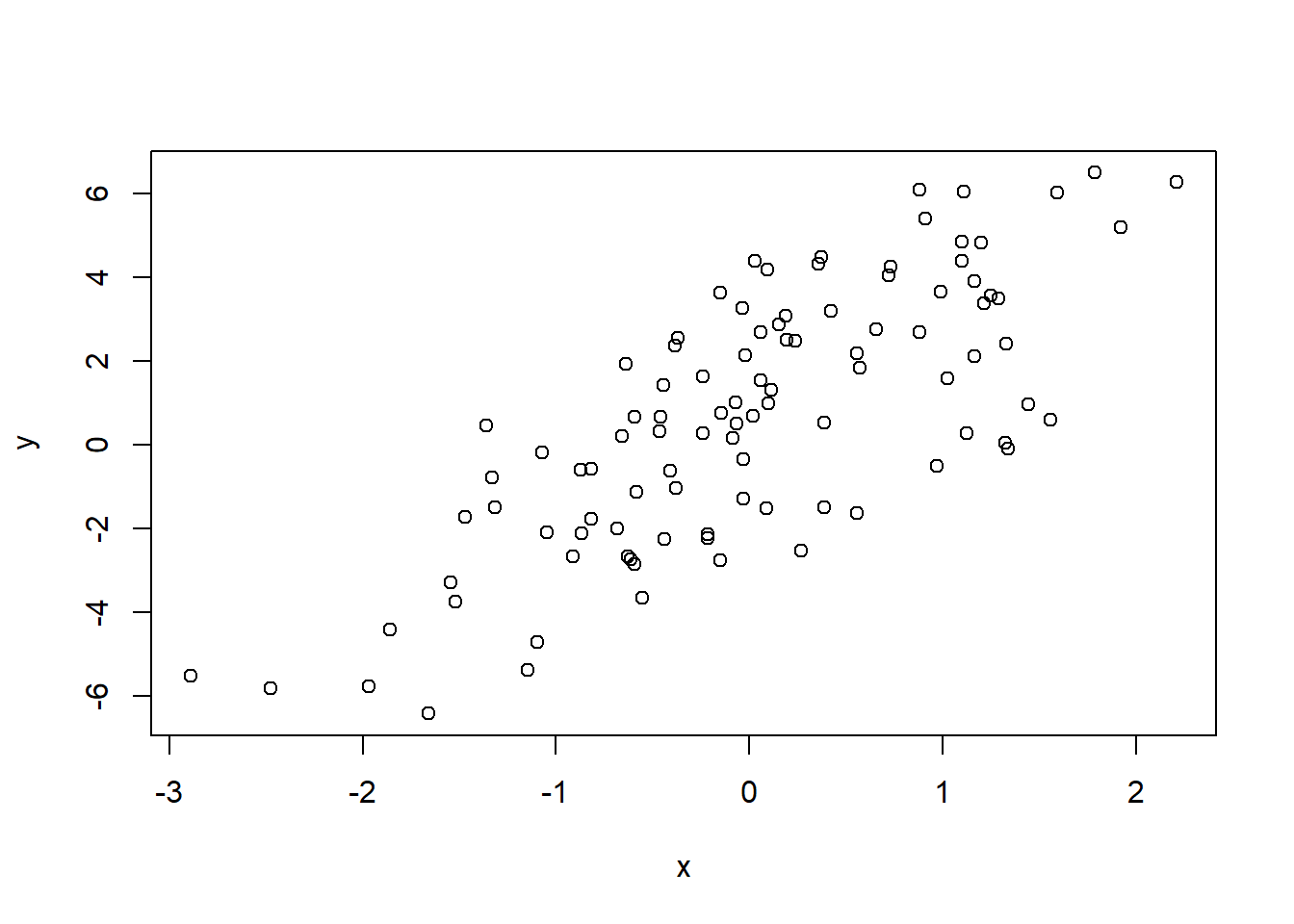

30.2 Random Sampling

The sample() function draws randomly from a specified set of (scalar) objects allowing you to sample from arbitrary distributions of numbers.

Example:

set.seed(1)
sample(1:10,4)

[1] 9 4 7 1

# Doesn't have to be numbers
sample(letters, 5)

[1] "b" "w" "k" "n" "r"

To sample more complicated things, such as rows from a dataframe or a list, you can sample the indices into an object rather than the elements of the object itself:

set.seed(20)
idx <- seq_len(nrow(airquality))## Create index vector 
samp <- sample(idx, 6) ##Sample from the index vector 
airquality[samp, ]

    Ozone Solar.R Wind Temp Month Day
107    NA      64 11.5   79     8  15
120    76     203  9.7   97     8  28
130    20     252 10.9   80     9   7
98     66      NA  4.6   87     8   6
29     45     252 14.9   81     5  29
45     NA     332 13.8   80     6  14