Regression analysis is a form of predictive modelling techniques that identifies the relationships between dependent and independent variables(s). The technique is used to find causal effect relationships between variables.
Regression analysis identifies the significant relationships between dependent and independent variables and the strength of the impact of multiple independent variables on dependent variables.
Linear Regressions
The linear regression equation is \(y = b_0 + b_1 x\) , where y is the dependent variable, x is the independent variable, \(b_0\) is the intercept, and \(b_1\) is the slope.
To use linear regression in R, you use the lm() function:
set.seed (123 )<- rnorm (100 , mean= 1 , sd= 1 )<- rnorm (100 , mean= 2 , sd= 2 )<- data.frame (x, y);<- lm (data$ y ~ data$ x, data= data)
Call:
lm(formula = data$y ~ data$x, data = data)

Coefficients:
(Intercept)       data$x
     1.8993      -0.1049
Call:
lm(formula = data$y ~ data$x, data = data)

Residuals:
   Min     1Q Median     3Q    Max
-3.815 -1.367 -0.175  1.161  6.581

Coefficients:
            Estimate Std. Error t value Pr(>|t|)
(Intercept)   1.8993     0.3033   6.261 1.01e-08 ***
data$x       -0.1049     0.2138  -0.491    0.625
---
Signif. codes:  0 '***' 0.001 '**' 0.01 '*' 0.05 '.' 0.1 ' ' 1

Residual standard error: 1.941 on 98 degrees of freedom
Multiple R-squared:  0.002453,  Adjusted R-squared:  -0.007726
F-statistic: 0.241 on 1 and 98 DF,  p-value: 0.6246
When the p-value is less than 0.05, the model is significant:
Furthermore:
The higher the R-squared and the adjusted R-squared , the better the linear model.
The lower the standard error , the better the model
Multiple Linear Regressions
Multiple linear regression is used when you have more than one independent variable.
The equation of a multiple linear regression is:
\(y = b_0 + b_1 x_1 + b_2 x_2 + ... + b_ k x_k + ϵ\)
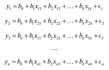
When you have n observations or rows in the data set, you have the following model:
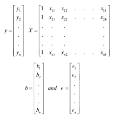
Using a matrix, you can represent the equations as: \(y = Xb + ϵ\)
To calculate the coefficients: ^b = (X’ X)-1 X’ y
set.seed (123 )<- rnorm (100 , mean= 1 , sd= 1 )<- rnorm (100 , mean= 2 , sd= 5 )<- rnorm (100 , mean= 2 , sd= 2 )<- data.frame (x, x2, y)<- lm (data$ y ~ data$ x + data$ x2, data= data)
Call:
lm(formula = data$y ~ data$x + data$x2, data = data)

Coefficients:
(Intercept)       data$x      data$x2
   2.517425    -0.266343     0.009525
Call:
lm(formula = data$y ~ data$x + data$x2, data = data)

Residuals:
    Min      1Q  Median      3Q     Max
-3.7460 -1.3215 -0.2489  1.2427  4.1597

Coefficients:
             Estimate Std. Error t value Pr(>|t|)
(Intercept)  2.517425   0.305233   8.248 7.97e-13 ***
data$x      -0.266343   0.209739  -1.270    0.207
data$x2      0.009525   0.039598   0.241    0.810
---
Signif. codes:  0 '***' 0.001 '**' 0.01 '*' 0.05 '.' 0.1 ' ' 1

Residual standard error: 1.903 on 97 degrees of freedom
Multiple R-squared:  0.01727,   Adjusted R-squared:  -0.00299
F-statistic: 0.8524 on 2 and 97 DF,  p-value: 0.4295