library(TSstudio)
data(USgas)
ts_plot(USgas,
        title = "US Monthly Natural Gas consumption",
        Ytitle = "Billion Cubic Feet",
Xtitle = "Year")36 Correlation Analysis
Due to the continuous and chronologically ordered nature of time series data, there is a likelihood that there will be some degree of correlation between the series observations. For instance, the temperature in the next hour is not a random event since, in most cases, it has a strong relationship with the current temperature or the temperatures that have occurred during the past 24 hours. In many cases, the series of past observations contains predictive information about future events, which can be utilized to forecast the series’ future observations.
36.1 Correlation Between Two Variables
One of the main goals of correlation analysis is to identify and quantify the relationship between two variables. This relationship could vary from having a full dependency or linear relationship between the two, to complete independence.
One of the most popular methods for measuring the level of correlation between two variables is the Pearson correlation coefficient. Although this method is not necessarily the most appropriate one for time series data, it is a simple and intuitive method for measuring correlation. This method, also known as the population correlation coefficient, is a ratio between the covariance of two variables and the multiplication of their standard deviation:
\[\begin{align*} \rho_{x,y}=\frac {COV(X,Y)}{\sigma_x \sigma_y} {, where -1\leq\rho_{x,y}\leq 1} \end{align*}\]
The values of the correlation coefficient segment the level of correlation into three main groups:
Positively correlated: This is where the value of the coefficient is greater than 0. This indicates some degree of a positive linear relationship between the variables, depending on the value of the coefficient. As the value of \(\rho_{x,y}\) (correlation coefficient) grows closer to 1, the linear relationship between the two variables grows stronger; 1 indicates a perfect linear dependency.
Negatively correlated: This is where the value of the coefficient is lower than 0. This is the reflection of the positive correlation, and it is an indication for an inverse linear relationship. In this case, as the value of \(\rho_{x,y}\) is closer to -1, the negative linear relationship of the two variables (for example, when one variable goes up the other goes down); -1 represents a perfect inverse linear dependency between the two variables.
Not correlated: This is where the value of the coefficient is equal to 0, which indicates that the two variables are independent.
Typically, we would consider the correlation between two variables to be strong if the value of the correlation coefficient is higher than 0.75 or lower than -0.75 (but this, of course, could change according to the field of research).
Measuring and analyzing the correlation between two variables, in the context of time series analysis, can be categorized in the following two categories:
Analyzing the correlation between a series and its lags, as some of the past lags may contain predictive information, which can be utilized to forecast future events of the series. One of the most popular methods for measuring the level of correlation between a series and its lags is the autocorrelation function.
Analyzing the correlation between two series (or causality analysis) in order to identify exogenous factors or predictors, which can explain the variation of the series over time (for example, the effect of weather patterns such as rainfall or temperature on taxi rides in New York City). In this case, the measurement of correlation is typically done with the cross-correlation function.
Note that while in lags analysis we extract the required data (the series lags) from the series itself, causality analysis requires additional effort, such as identifying and extracting external variables, which may not always available.
36.2 Lags Analysis
The goal of lags analysis is to identify and quantify the relationship between a series and its lags. This relationship is typically measured by calculating the correlation between the two and with the use of data visualization tools.
Example 1:
Note that one of the main characteristic of the USgas series is the strong seasonal pattern.
Example 2:
data(EURO_Brent)
ts_plot(EURO_Brent,
        title = "Brent Crude Oil Prices",
        Ytitle = "US Dollars per Barrel",
        Xtitle = "Year")
As you can see the EURO_Brent series plot, which represents the monthly prices of the Brent crude oil in USD, the price of the oil does not have seasonal patterns or general trends.
Example 3:
data(USVSales)
ts_plot(USVSales,
        title = "US Monthly Total Vehicle Sales",
        Ytitle = "Thousands of units",
        Xtitle = "Year")
The plot of USVSales, the US monthly total vehicle sales, is an example of a series with both seasonal and cycle patterns.
36.2.1 The autocorrelation function
The autocorrelation function (ACF) is the main method in time series analysis for quantifying the level of correlation between a series and its lags. The acf function from the stats package is R’s built-in ACF, which, by default, visualizes the results using a bar plot.
Example 1:
Use the acf function to plot the correlation of the USgas series and its first 60 lags (by setting the lag.max argument to 60)
acf(USgas, lag.max = 60)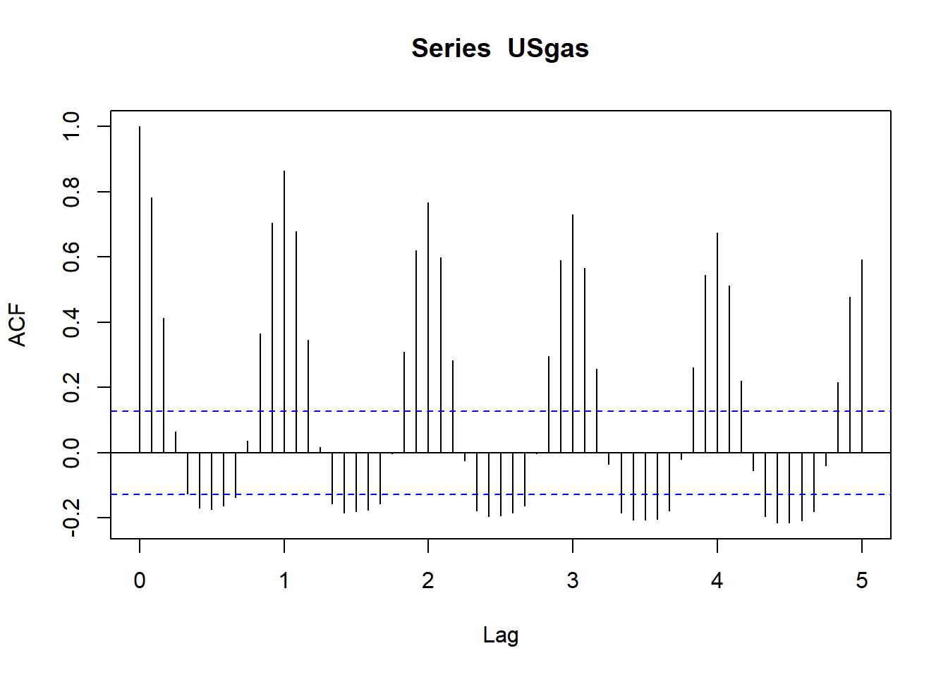
Each bar in the ACF plot represents the level of correlation between the series and its lags in chronological order. Note that according to the x-axis notation lags 1 and 2 represent the 12 and 24 lags. The blue dotted lines indicate whether the level of correlation between the series and each lag is significant or not. By testing the null hypothesis that the correlation of the lag with the series is equal to zero, we can reject it whenever the level of correlation is either above or below the upper and lower dotted lines, respectively, with a level of significance of 5%. Otherwise, whenever the correlation is between the upper and lower dotted lines, we fail to reject the null hypothesis, and we can therefore ignore those lags (or assume that there is no significant correlation between the two).
As you can see from the USgas ACF plot, the series has a strong positive correlation with the seasonal lags (which decay over time) along with negative correlation with the mid-seasonal lags (for example, lags 6, 18, and 30).
Example 2:
acf(EURO_Brent, lag.max = 60)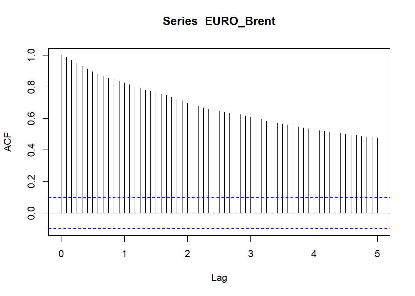
You can see that the correlation of the series with its lags is decaying over time, whereas the closer the lag is, chronologically to the series, the stronger the relationship with the series. This type of correlation is also an indication that the series is not stationary and a differencing of the series is required.
Example 3:
acf(USVSales, lag.max = 60)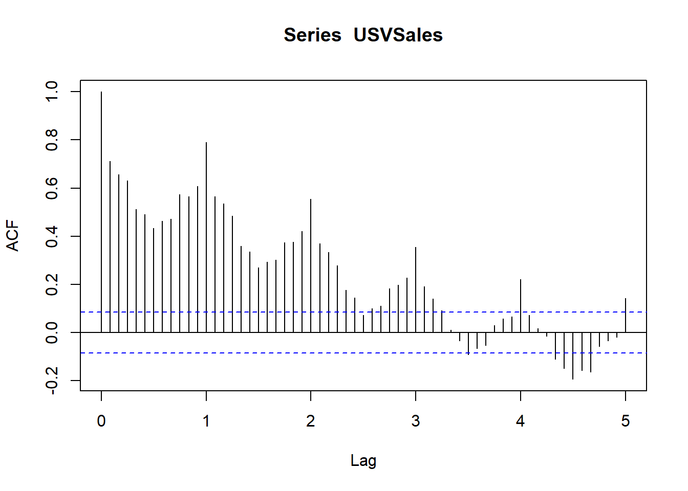
The correlation plot has a cyclic shape as a result of the seasonal pattern of the series. On the other hand, the decay rate of USVSales is faster compared to the rate of USgas due to the cycle pattern of the series, which shifts the series direction over time. As a result, the series is mainly correlated with the first seasonal lag. That being said, if we remove the series cycle (or detrend it) we will probably have a similar correlation pattern as USgas.
36.2.2 Lag plots
A lag plot is a non-statistical approach for analyzing the relationship between a series and its lags. This method is based on data visualization tools, with the use of two-dimensional scatter plots for visualizing the series (typically on the y-axis) against the \(k\) lag of the series. Hence, each pair of points represents a combination of the series observations and their corresponding lagged values. As more points on the lag plot are closer to the 45 degree line, the higher the correlation will be between the series and the corresponding lag.
Example 1:
ts_lags(USgas)You can see that, moving along from the first lag up to the sixth lag, the relationship between the series and its lags become less linear. This process starts to reverse from the seventh lag as the relationship gradually becomes more linear, where the seasonal lag (or lag 12) has the strongest relationship with the series. Those results are aligned with the ones we saw earlier with the ACF plot.
# Plot the most recent seasonal lags (that is, lags 12, 24, 36, and 48)
ts_lags(USgas, lags = c(12, 24, 36, 48))
Example 2:
ts_lags(EURO_Brent)As you can see, the results are aligned with the ones we received before with the ACF. The EURO_Brent series has a strong linear relationship with the first lag, where the strength of that relationship decays as the distance of the lag from the series is higher.
Example 3:
ts_lags(USVSales)In the case of USVSales, the 12 lag has the closest linear relationship with the series (as we observed before with the ACF plot).
36.3 Causality Analysis
The goal of causality analysis, in the context of time series analysis, is to identify whether a causality relationship exists between the series we wish to forecast and other potential exogenous factors. The use of those external factors as drivers of the forecasting model (whenever exists) could potentially provide accurate and robust forecast (as oppose of using only the past observation of the series).
36.3.1 Causality vs correlation
Two variables will have a causality relationship whenever the change of one variable triggers a direct change of the second variable. This is also known as a cause-and-effect. For instance, the temperatures in Chicago have a direct impact on the consumption of natural gas throughout the year (as most of the heating systems operate with natural gas) and we can therefore assume that there is a causality relationship between the two. One of the main characteristics of causality is a high correlation between the two variables.
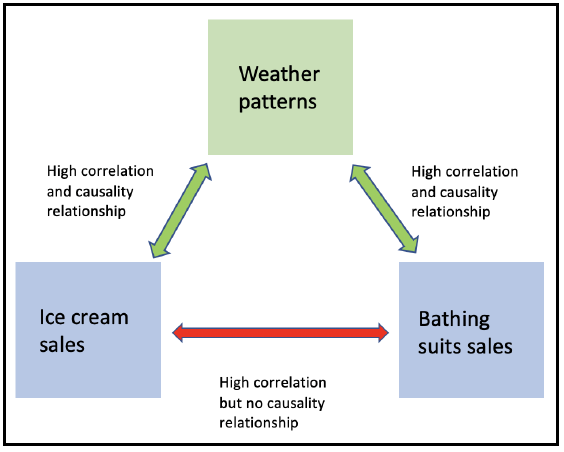
However, this could be misleading in some cases, as high correlation by itself between two variables should not instantly imply the existence of a causality relationship, as the two may have a high dependency on a third variable. For example, you should expect to have a high correlation between the sales of ice cream and bathing suits (high demand during the summer and low throughout the winter), but there is no causal relationship between the two besides the fact that both are highly correlated with the same factor —the season of the year (or weather patterns).
The following diagram describes this type of relationship:
In the context of time series analysis, the causality between two time series can be categorized into the following two types:
Direct causality: This is where series B reacts immediately to the changes of series A at time t. For example, the speed of the wind will have a direct impact on the level of electricity production of a wind turbine.
In-direct causality: This is where the change of series A at time t triggers a change of series B at time t + n (where n > 0). This lag effect is common in economic indicators, such as Gross Domestic Product (GDP) and consumption or the unemployment rate, where the change in the first triggers a gradual change in the other over time (for example, a drop in the GDP this quarter will impact the employment rate in the next quarter).
Typically, a series from the first type will have a stronger dependency and a higher level of correlation compared to the second type. Yet, it is harder (or even not practical in some cases) to utilize series A as a predictor of series B, as the future values of series A are unknown and therefore need to be forecast as well (unless the future values are deterministic).
This could potentially increase the level of uncertainty of the model output, due to the fact that the input values are forecasted and will therefore come with some degree of uncertainty (as opposed to the actual input values of series A that were used in the training process). For example, if you wish to forecast the level of electricity production of a wind turbine during the next 10 days by using the wind speed as a predictor, you will have to forecast the wind speed in the next 10 days as well.
In conclusion, analyzing and identifying causality between two series is based on the use of correlation measurement and lag plots, along with some intuition and common sense (as mentioned previously, high correlation by itself is not necessarily an indication for causality).
36.3.2 The cross-correlation function
The cross-correlation function (CCF) is the sister function of the ACF and it measures the level of correlation between two series and their lags in a fairly similar way.
Example:
Analyze the relationship between the total vehicle sales (USVSales) and the unemployment rate (USUnRate) in the US to understand whether there is a cause and effect relationship between the two.
data(USUnRate)
ts_plot(USUnRate,
        title = "US Monthly Civilian Unemployment Rate",
        Ytitle = "Unemployment Rate (%)",
        Xtitle = "Year")
However, as the USUnRate series starts during the 1950s, as opposed to the USVSales series, which began in 1976, we need before starting to align the two series to the same time frame using the window function:
us_vsales <- window(USVSales, start = c(1976,1), end = c(2018,6))
us_unrate <- window(USUnRate, start = c(1976,1), end = c(2018,6))
Next, we will plot the two series on a two-y-axis plot (as the units of the two series are different) using the plotly package:
library(plotly)
plot_ly(x = time(us_vsales),
        y = us_vsales,
        type = "scatter",
        mode = "line",
        name = "Total Vehicle Sales") %>%
  add_lines(x = time(us_unrate),
            y = us_unrate,
            name = "Unemployment Rate",
            yaxis = "y2") %>%
  layout(title = "Total Monthly Vehicle Sales vs Unemployment Rate in the US",
         yaxis2 = list(overlaying = "y",
                       side = "right",
                       title = "Percentage",
                       showgrid = FALSE),
         yaxis = list(title = "Thousands of Units",
                      showgrid = FALSE),
         legend = list(orientation = 'h'),
         margin = list(l = 50, r = 50, b = 50, t = 50, pad = 2))
From the preceding plot one can see that the two series move to the opposite direction, so when the vehicle sales increase, the unemployment rate decreases and the other way around. You can also see that, in most of the cases, the changes in the vehicle sales series are leading to the changes in the unemployment rate.
To explore this assumption further, we can measure the level of correlation between the unemployment rate and the vehicle sales and its lags using the ccf function from the stats package as well:
Example:
ccf(x = us_vsales, y = us_unrate, lag.max = 36)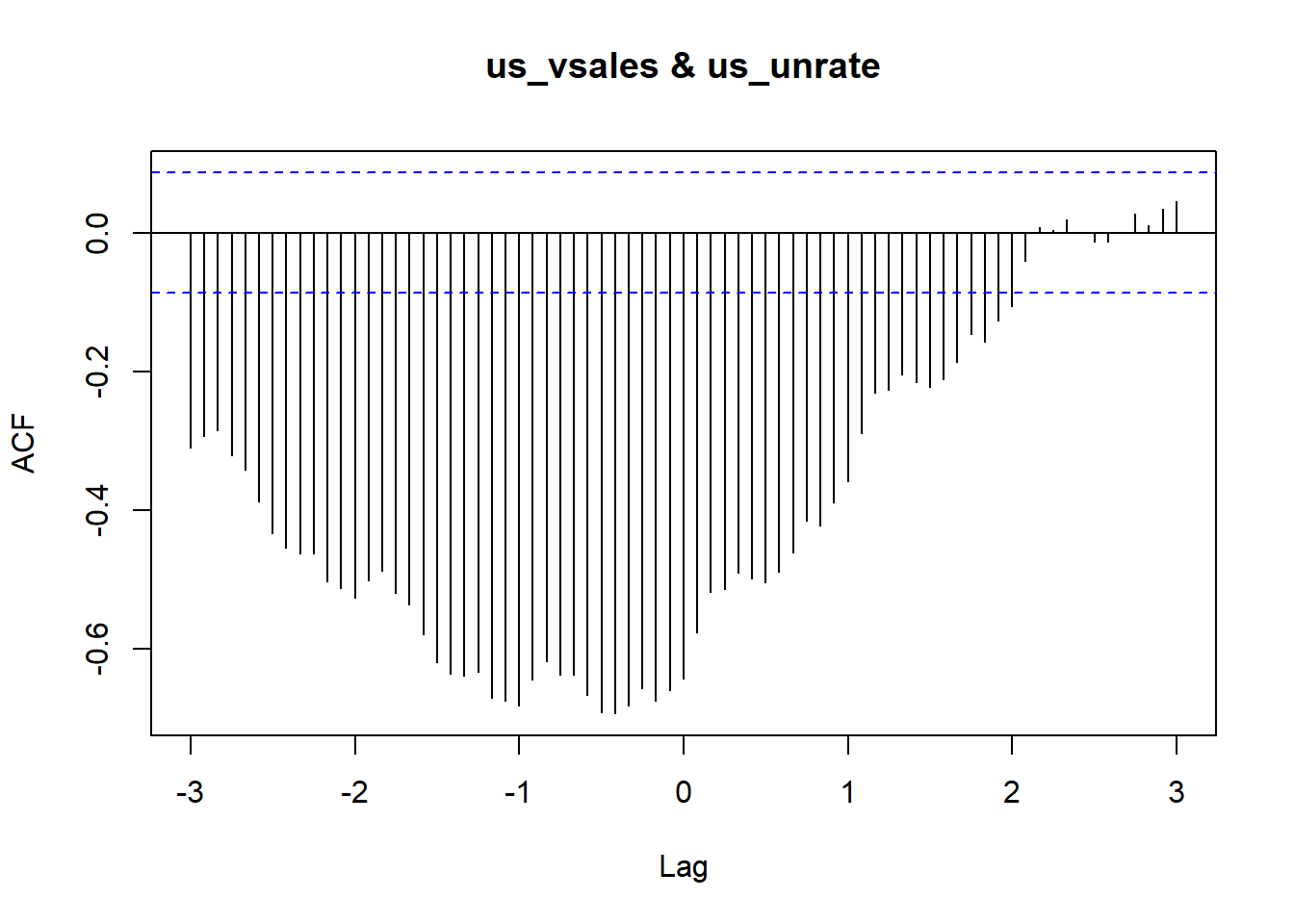
Similarly to the ACF output, each bar in the CCF plot represents the level of correlation between the main series and the lags of the secondary. Lag 0 represents the direct correlation between the two (original) series, where the negative and positive lags represent the correlation between the unemployment rate and the past and leading lags of the vehicle sales series, respectively. The main thing to note from the preceding plot is that the unemployment rate is correlated more to the past lags as opposed to the leading lags of the vehicle sales.
It is difficult (and probably even wrong) to conclude from the results that the vehicle sales explicitly drive the changes in the unemployment rate (and it is definitely not in the scope of this book). However, there is some indication of a causality relationship, which can be derived from the level of correlation along with common sense, given the size of the vehicle industry in the US and its historical impact on the economy.
Alternatively, you can plot the relationship between US vehicle sales and the lags of the unemployment rate with the ccf_plot function from the TSstudio package. This function works similarly to the ts_lags function we previously introduced:
ccf_plot(x = USVSales, y = USUnRate, lags = 0:12)The main advantage of the ccf_plot function over the ccf function is that the first automatically aligns the two series according to their chronological order, whereas the ccf function does not have this automatic functionality, and therefore requires a pre-processing step (as we used previously with the window function).