14 Descriptive Statistics

Descriptive statistics summarizes the data set, lets us have a feel and understanding of the data and variables. Descriptive statistics usually focuses on:

the distribution: can be a normal distribution, binomial distribution, and other distributions like Bernoulli distribution.
the central tendency: can be the mean, median, and mode of the data.
the dispersion of the data: it describes the spread of the data, and dispersion can be the variance, standard deviation, and interquartile range.

Descriptive statistics allows us to decide or determine whether we should use inferential statistics to identify the relationship between data sets, or use regression analysis instead to identify the relationships between variables.

14.1 `summary()` and `str()`

The summary() and str() functions are the fastest ways to get descriptive statistics of the data.

The summary() function gives the basic descriptive statistics of the data.
The str() function gives the structure of the variables.

14.2 Measures of Centrality

14.2.1 Mode

The mode is a value in data that has the highest frequency:

Example:

a <- c(1, 2, 3, 4, 5, 5, 5, 6, 7, 8)
# To get mode in a vector you create a frequency table
(y <- table(a))

a
1 2 3 4 5 6 7 8 
1 1 1 1 3 1 1 1

names(y)[which(y==max(y))]

[1] "5"

14.2.2 Median

The median is the middle or midpoint of the data and is also the 50 percentile of the data.

The median is affected by the outliers and skewness of the data.

median(a)

[1] 5

14.2.3 Mean

The mean is the average of the data. The mean works best if the data is distributed in a normal distribution or distributed evenly.

mean(a)

[1] 4.6

14.3 Measures of Variability

The measures of variability are the measures of the spread of the data. These are encompasses:

Variance.
Standard deviation.
Range.
Interquartile range.
and more.

14.3.1 Variance

The variance is the average of squared differences from the mean, and it is used to measure the spreadness of the data:

Population variance:

A <- c(1, 2, 3, 4, 5, 5, 5, 6, 7, 8)
N <- length(A)
var(A) * (N - 1) / N

[1] 4.24

Sample variance:

var(A)

[1] 4.711111

14.3.2 Standard deviation

The standard deviation is the square root of a variance and it measures the spread of the data.

Population standard deviation:

A <- c(1, 2, 3, 4, 5, 5, 5, 6, 7, 8)
N <- length(A)
variance <- var(A) * (N - 1) / N
sqrt(variance)

[1] 2.059126

Sample standard deviation:

sd(A)

[1] 2.170509

14.3.3 range()

The range is the difference between the largest and smallest points in the data:

range(A)

[1] 1 8

res <- range(A)
diff(res)

[1] 7

min(A)

[1] 1

max(A)

[1] 8

14.3.4 Interquartile Range

The interquartile range is the measure of the difference between the 75 percentile or third quartile and the 25 percentile or first quartile.

IQR(A)

[1] 2.5

You can get the quartiles by using the quantile() function:

quantile(A)

  0%  25%  50%  75% 100% 
1.00 3.25 5.00 5.75 8.00

14.4 Distributions

14.4.1 Normal Distribution

If the points do not deviate away from the line, the data is normally distributed.

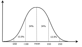
To see whether data is normally distributed, you can use the qqnorm() and qqline() functions:

qqnorm(data$x) #You must first draw the distribution to draw the line afterwards 
qqline(data$x)

You can also use a Shapiro Test to test whether the data is normally distributed. If the p-value is more than 0.05, you can conclude that the data does not deviate from normal distribution:

shapiro.test(data$x)

14.4.2 Modality

The modality of a distribution can be seen by the number of peaks when we plot the histogram.

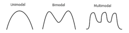
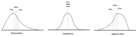
Figure 2: The modality of a distribution

14.4.3 Skewness

Skewness is a measure of how symmetric a distribution is and how much the distribution is different from the normal distribution.

Negative skew is also known as left skewed, and positive skew is also known as right skewed: - A positive skewness indicates that the size of the right-handed tail is larger than the left-handed tail. - A negative skewness indicates that the left-hand tail will typically be longer than the right-hand tail.

The Pearson’s Kurtosis measure is used to see whether a dataset is heavy tailed, or light tailed. High kurtosis means heavy tailed, so there are more outliers in the data.

When kurtosis is close to 0, then a normal distribution is often assumed. These are called mesokurtic distributions.
When kurtosis>0, then the distribution has heavier tails and is called a leptokurtic distribution.
When kurtosis<0, then the distribution is light tails and is called a platykurtic distribution.

To find the kurtosis and skewness in R, you must install the moments package:

install.packages("moments")
skewness(data$x)
kurtosis(data$x)

14.4.4 Binomial Distribution

A binomial distribution has two outcomes, success or failure, and can be thought of as the probability of success or failure in a survey that is repeated various times.

dbinom(32, 100, 0.5)

[1] 0.000112817

14.1 summary() and str()