As with other fields of statistics and, in particular, the field of machine learning, one of the primary goals of time series analysis is to identify patterns in data. Those patterns can then be utilized to provide meaningful insights about both past and future events, such as seasonal, outliers, or unique events.
Patterns in time series analysis can be categorized into one of the following:
Structural patterns: These are also known as series components, which represent the core structure of the series. There are three types:
Structural patterns—trend.
Cycle.
Seasonal.
You can think about those patterns as binary events, which may or may not exist in the data. This helps to classify the series characteristics and identify the best approach to analyze the series.
Non-structural: This is also known as the irregular component, and refers to any other types of patterns in the data that are not related to the structural patterns.
We can use these two groups of patterns (structural and non-structural) to express time series data using the following equation, when the series has an additive structure:
Where \(Y_{t}\) represents the series observation at time \(t\) and \(T_{t}\), \(S_{t}\), \(C_{t}\), and \(I_{t}\) represent the value of the trend, seasonal, cycle, and irregular components of the series at time \(t\), respectively. You can learn more in this section.
33.1 The Cycle Component
A cycle can be described as a sequence of repeatable events over time, where the starting point of a cycle is at a local minimum of the series and the ending point is at the next one, and the ending point of one cycle is the starting point of the following cycle. Unlike the seasonal pattern, cycles do not necessarily occur at equally spaced time intervals, and their length could change from cycle to cycle.
Example:
library(TSstudio)data(USUnRate)ts_info(USUnRate)
 The USUnRate series is a ts object with 1 variable and 864 observations
 Frequency: 12
 Start time: 1948 1
 End time: 2019 12
Looking at the preceding series plot, you can observe that the series has had three cycles since 1990 of different length:
The first cycle occurred between 1990 and 2000, which was close to an 11-year cycle.
The second cycle started in 2000 and ended in 2007, which was a 7-year cycle.
A third cycle, which began in 2007 and as of May 2019 has not been completed yet, which means that this has continued for more than 12 years.
33.2 The Trend Component
A trend, if it exists in time series data, represents the general direction of the series, either up or down, over time. Furthermore, a trend could have either linear or exponential growth (or close to either one), depending on the series characteristics.
Example:
These examples represent time series data with a clear trend component, and it is therefore easy to identify the trend and classify its growth type.
33.3 The Seasonal Component
The seasonal component (or seasonality) is another common pattern in time series data. If it exists, it represents a repeated variation in the series, which is related to the frequency units of the series (for example, the months of the year for a monthly series).
A common examples for a series with a strong seasonality pattern is the demand for electricity or natural gas. In those cases, the seasonal pattern is derived from a variety of seasonal events, such as weather patterns, the season of the year, and sunlight hours.
Example:
The seasonal and cycle components both describe cyclic events over time, where the length of their cycle distinguish the two. The seasonal component has a constant cycle, which is derived and tied to the series frequency. On the other hand, the cycle length of the cycle component is not necessarily constant and can typically vary from one cycle to the next one.
A common way to identify whether a cycle pattern exists in a series is with the use of a heatmap for the time series data.
Example:
ts_heatmap(USgas,title ="Heatmap - the US Natural Gas Consumption")
33.4 White Noise
A series is defined as white noise when there is no correlation between the series observations or patterns. In other words, the relationship between different observations is random. Typically, unless mentioned otherwise, we assume that white noise is an independent and identically distributed random.
Example:
There are a few methods for testing whether a time series is white noise:
The basic method is carried out by plotting and eyeballing the series to identify whether the variation of the series appears to be random or not.
We can measure the correlation between the series and its lags with the autocorrelation function (ACF). A series is considered to be white noise whenever there is no correlation between the series and its lag. The acf function from the stats package calculates the level of correlation between a series and its lags.
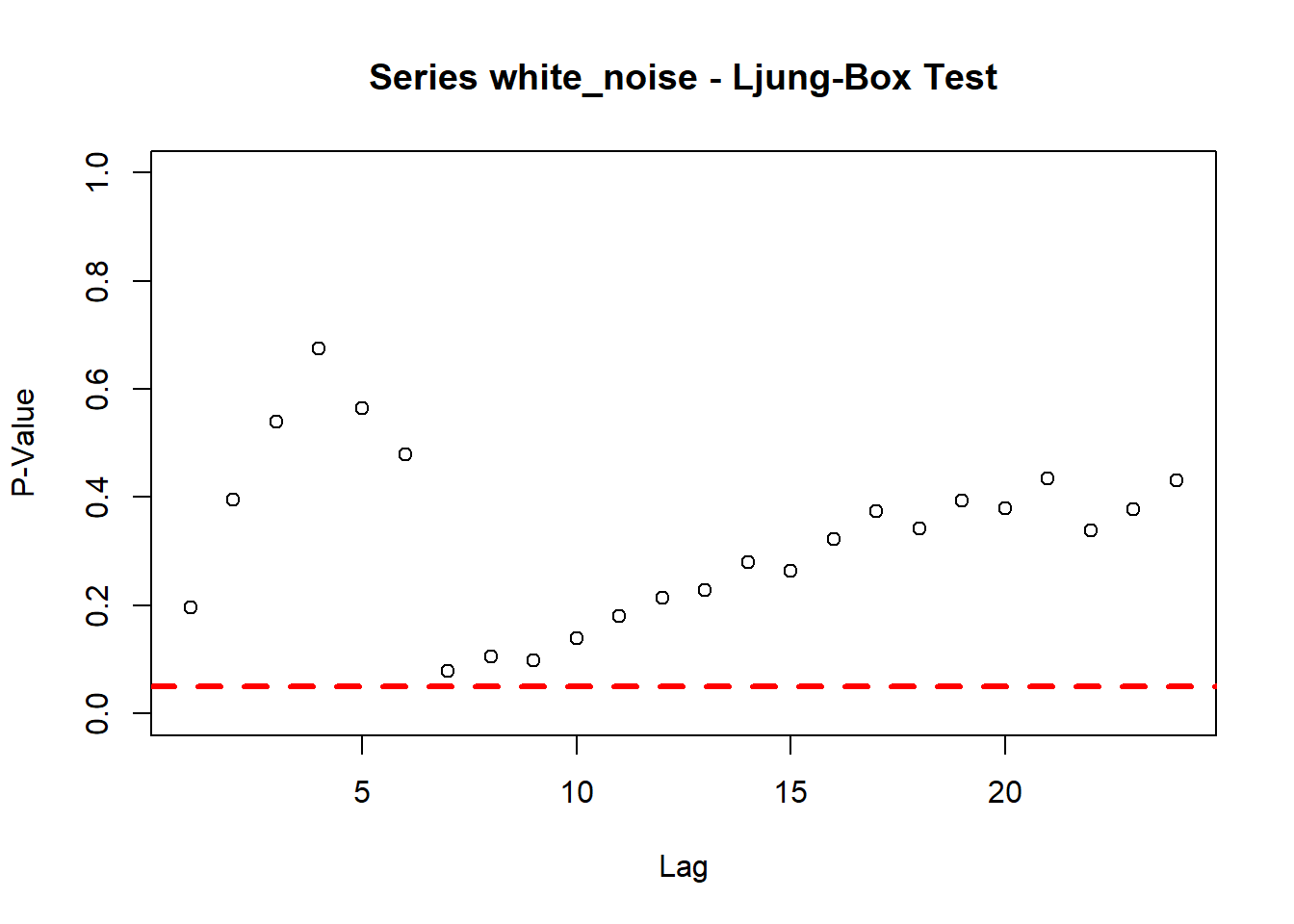
The Ljung-Box test is another statistical test to evaluate whether the series is correlated with its lags. In this case, the null hypothesis assumes that the lags are not correlated. Therefore, lags with lower p-values (with respect to the level of significance of the test) would be considered as being correlated with the series. The Box.testfunction, another stats package function, performs a Ljung-Box test on a series and a specific lag.
Example:
library(dplyr)x <-lapply(1:24, function(i){ p <-Box.test(white_noise, lag = i, type ="Ljung-Box") output <-data.frame(lag = i, p_value = p$p.value)return(output) }) %>% bind_rowsplot(x = x$lag,y = x$p_value, ylim =c(0,1),main ="Series white_noise - Ljung-Box Test",xlab ="Lag", ylab ="P-Value")abline(h =0.05, col="red", lwd=3, lty=2)
You can see in the preceding Ljung-Box test summary that the p-value of all the lags is above the red dotted line, which indicates that we failed to reject the null hypothesis for a level of significance of 0.05. This indicates that the series is not correlated with its first 24 lags and is, therefore, a white noise series.
33.5 The Irregular Component
This component is the remainder between the series and structural components, and provides an indication of irregular events in the series. This includes non-systematic patterns or events in the data, which cause irregular fluctuation. In addition, the irregular component could provide some indication of the appropriate fit of the other components when using a decomposing method.
A high correlation in this component is an indication that some patterns related to one of the other components were leftover due to an inaccurate estimate. On the other hand, if the irregular component is not correlated with its lags (that is, a white noise), we can assume (depending on the series structure) that the estimation of the trend and seasonal components captured the majority of the information about the series structure.
33.6 The Additive versus the Multiplicative Model
These terms describe the model structure. A model is defined as additive whenever we add together its components, namely, whenever there is a growth in the trend (with respect to the previous period), or if the amplitude of the seasonal component roughly remains the same over time:
The US monthly natural gas consumption series is an example of an additive series. You can easily notice that the amplitude of the seasonal component remains the same (or close to the same) over time:
As you can see, the amplitude of the USgas series seasonal component over the past 20 years did not change by much (apart from some years, which may be related to some unusual weather patterns). In addition, the series trend seems to be linear, with some structural breaks during 2010.
Similarly, a model is defined as multiplicative whenever we multiply its components, namely, whenever the growth of the trend or the magnitude of the seasonal component increases or decreases by some multiplicity from period to period over time:
The AirPassengers dataset (available in the dataset package), which describes the total monthly international airline passengers between the years 1949 and 1960, is an example for multiplicative series. As you can see in the following data, the amplitude of the seasonal component increases from year to year:
The typical approach for handling a series with a multiplicative structure is by applying a data transformation on the input series. The most common data transformation approaches for time series data are the following:
Log transformation: This applies a log on both sides of the series equation. The new structure of the series allows us to treat it as a normal additive series:
As you can see from the preceding Box-Cox equation, for \(\lambda=0\), the transformation is a log transformation.
The forecast package provides several tools for applying a Box-Cox transformation on time series data. The BoxCox.lambda function estimates the value of \(\lambda\), which minimizes the coefficient variation of the input series.
Example:
We will use BoxCox.lambda to identify the \(\lambda\) value for the AirPassenger series:
As you can see from the transformation plot of the AirPassenger series, the values of the series are scaled. Note that most of the forecasting models in the forecast package automatically transform the series before applying the model, and then re-transform the forecast output back to the original scale.