library(TSstudio)
ts_info(USVSales)
The USVSales series is a ts object with 1 variable and 528 observations
Frequency: 12
Start time: 1976 1
End time: 2019 12 In recent years, the use of machine learning (ML) models has become popular and accessible due to significant improvement in standard computation power. This led to a new world of methods and approaches for regression and classifications models.
The main advantage of the ML models is their predictive power (when quality inputs are available), which, in many cases, is worth the effort and time involved in the process. In the context of time series forecasting, it will be beneficial to forecast with ML models in the following cases:
Structural patterns: Exits in the series, as those can produce new, predictive features.
Multiple seasonality: As a special case for structural patterns since, typically, the traditional time series models are struggling to capture those patterns when they exist.
In this section, we will focus on exploring and learning about the main characteristics of the USVSales series. These insights will be used to build new features as inputs for the ML model. The exploratory analysis of the USVSales series will focus on the following topics:
Let’s start with ts_info and review the structure of the USVSales series:
Example
library(TSstudio)
ts_info(USVSales) The USVSales series is a ts object with 1 variable and 528 observations
Frequency: 12
Start time: 1976 1
End time: 2019 12 The USVSales series is a monthly ts object which represents the total vehicle sales in the US between 1976 and 2018 in thousands of units. Let’s plot the series and review its structure with the ts_plot function:
ts_plot(USVSales,
        title = "US Total Monthly Vehicle Sales",
        Ytitle = "Thousands of Units",
        Xtitle = "Year")
As you can see in the preceding plot, the series has cycle patterns, which is common for a macro economy indicator. In this case, it is a macro indicator of the US economy.
We can get a deeper view of the series components by decomposing the series into its components and plotting them with the ts_decompose function:
ts_decompose(USVSales)Beside the cycle-trend component, we can observe that the plot has a strong seasonal pattern, which we will explore next.
To get a closer look at the seasonal component of the series, we will subtract from the series, decompose the trend we discussed previously, and use the ts_seasonal function to plot the box plot of the seasonal component of the detrend series:
USVSales_detrend <- USVSales - decompose(USVSales)$trend
ts_seasonal(USVSales_detrend, type = "box")
We can see from the preceding seasonal plot that, typically, the peak of the year occurred during the months of March, May, and June. In addition, you can see that the sales decay from the summer months and peak again in December during the holiday seasons. On the other hand, the month of January is typically the lowest month of the year in terms of sales.
The USVSales series has a high correlation with its first seasonal lag. We can review this assessment with the use of the ts_acf function from the TSstudio package for reviewing the autocorrelation of the series:
# `ts_cor`substitutes ts_acf
ts_cor(USVSales)
We can zoom in on the relationship of the series with the last three seasonal lags using the ts_lags function:
ts_lags(USVSales, lags = c(12, 24, 36))The relationship of the series with the first and also second seasonal lags has a strong linear relationship, as shown in the preceding lags plot.
We can conclude our exploratory analysis of the USVSales series with the following observations:
The USVSales series is a monthly series with a clear monthly seasonality.
The series trend has a cyclic shape, and so the series has a cycle component embedded in the trend.
The series’ most recent cycle starts right after the end of the 2008 economic crisis, between 2009 and 2010.
It seems that the current cycle reached its peak as the trend starts to flatten out.
The series has a strong correlation with its first seasonal lag.
Moreover, as we intend to have a short-term forecast (of 12 months), there is no point in using the full series, as it may enter some noise into the model due to the change of the trend direction every couple of years. (If you were trying to create a long-term forecast, then it may be a good idea to use all or most of the series.)
Therefore, we will use the model training observations from 2010 and onward. We will use the ts_to_prophet function from the TSstudio package to transform the series from a ts object into a data.frame, and the window function to subset the series observations since January 2010:
df <- ts_to_prophet(window(USVSales, start = c(2010,1)))
names(df) <- c("date", "y")
head(df)
date y
1 2010-01-01 712.469
2 2010-02-01 793.362
3 2010-03-01 1083.953
4 2010-04-01 997.334
5 2010-05-01 1117.570
6 2010-06-01 1000.455Before we move forward and start with the feature engineering stage, let’s plot and review the subset series of USVSales with the ts_plot function:
ts_plot(df, title = "US Total Monthly Vehicle Sales (Subset)",
        Ytitle = "Thousands of Units",
Xtitle = "Year")Feature engineering plays a pivotal role when modeling with ML algorithms. Our next step, based on the preceding observations, is to create new features that can be used as informative input for the model. In the context of time series forecasting, these are some examples of possible new features that can be created from the series itself:
The series trend: This uses a numeric index. In addition, as the series trend isn’t linear, we will use a second polynomial of the index to capture the overall curvature of the series trend.
Seasonal component: This creates a categorical variable for the month of the year to capture the series’ seasonality.
Series correlation: This utilizes the strong correlation of the series with its seasonal lag and uses the seasonal lag (lag12) as an input to the model.
Example:
library(dplyr)
library(lubridate)
df <- df %>% mutate(month = factor(month(date, label = TRUE),
                                   ordered = FALSE),
                    lag12 = lag(y, n = 12)) %>%
  filter(!is.na(lag12))
# Add the trend component and its second polynomial (trend squared)
df$trend <- 1:nrow(df)
df$trend_sqr <- df$trend ^ 2
# View the structure of the df object after adding the new features
str(df)
'data.frame': 108 obs. of 6 variables:
$ date : Date, format: "2011-01-01" "2011-02-01" ...
$ y : num 836 1007 1277 1174 1081 ...
$ month : Factor w/ 12 levels "ene","feb","mar",..: 1 2 3 4 5 6 7 8 9 10 ...
$ lag12 : num 712 793 1084 997 1118 ...
$ trend : int 1 2 3 4 5 6 7 8 9 10 ...
$ trend_sqr: num 1 4 9 16 25 36 49 64 81 100 ...There are additional feature engineering steps, which in the case of the USVSales series are not required, but may be required in other cases, i.e. scaling, hot encoding.
In order to compare the different models that we will be testing in this chapter, we will use the same inputs that we used previously. This includes executing same training and testing partitions throughout this chapter. Since our forecast horizon is for 12 months, we will leave the last 12 months of the series as testing partitions and use the rest of the series as a training partition:
h <- 12
train_df <- df[1:(nrow(df) - h), ]
test_df <- df[(nrow(df) - h + 1):nrow(df), ]
Previously, the \(h\) variable represented the forecast horizon, which, in this case, is also equal to the length of the testing partition. We will evaluate the model’s performance based on the MAPE score on the testing partition.
Be aware that One of the main characteristics of ML models is the tendency to overfit on the training set. Therefore, you should expect that the ratio between the error score on the testing and training partition will be relatively larger than the corresponding results of traditional time series models, such as ARIMA, Holt-Winters, and time series linear regression. In addition to the training and testing partitions, we need to create the inputs for the forecast itself. We will create a data.frame with the dates of the following 12 months and build the rest of the features:
forecast_df <- data.frame(date = seq.Date(from = max(df$date) + month(1),
                                          length.out = h, by = "month"),
                          trend = seq(from = max(df$trend) + 1,
                                      length.out = h, by = 1))
forecast_df$trend_sqr <- forecast_df$trend ^ 2
forecast_df$month <- factor(month(forecast_df$date, label = TRUE),
                            ordered = FALSE)
Last but not least, we will extract the last 12 observations of the series from the df object and assign them as the future lags of the series:
forecast_df$lag12 <- tail(df$y, 12)The performance of a forecasting model should be measured by the error rate, mainly on the testing partition, but also on the training partition. You should evaluate the performance of the model with respect to some baseline model. Since we are using a family of ML regression models, it makes more sense to use a regression model as a benchmark for the ML models.
We will train a time series linear regression model using the training and testing partitions we created previously, and evaluate its performance with the testing partitions:
lr <- lm(y ~ month + lag12 + trend + trend_sqr, data = train_df)
summary(lr)
Call:
lm(formula = y ~ month + lag12 + trend + trend_sqr, data = train_df)

Residuals:
     Min       1Q   Median       3Q      Max
-146.625  -38.997    0.111   39.196  112.577

Coefficients:
             Estimate Std. Error t value Pr(>|t|)
(Intercept) 542.93505   72.59490   7.479 7.91e-11 ***
monthfeb    112.73160   34.16141   3.300 0.001439 **
monthmar    299.20932   54.24042   5.516 4.03e-07 ***
monthabr    182.52406   42.53129   4.292 4.88e-05 ***
monthmay    268.75603   51.28464   5.240 1.24e-06 ***
monthjun    224.66897   44.26374   5.076 2.41e-06 ***
monthjul    177.88564   42.21898   4.213 6.49e-05 ***
monthago    241.63260   47.00693   5.140 1.86e-06 ***
monthsep    152.99058   37.04199   4.130 8.76e-05 ***
monthoct    125.16484   35.04896   3.571 0.000601 ***
monthnov    127.97288   34.18772   3.743 0.000338 ***
monthdic    278.67994   51.09552   5.454 5.21e-07 ***
lag12         0.33906    0.10738   3.158 0.002236 **
trend         7.73667    1.72415   4.487 2.36e-05 ***
trend_sqr    -0.05587    0.01221  -4.576 1.69e-05 ***
---
Signif. codes:  0 '***' 0.001 '**' 0.01 '*' 0.05 '.' 0.1 ' ' 1

Residual standard error: 59.6 on 81 degrees of freedom
Multiple R-squared:  0.9198,    Adjusted R-squared:  0.9059
F-statistic: 66.36 on 14 and 81 DF,  p-value: < 2.2e-16
Next, we will predict the corresponding values of the series on the testing partition with the predict function by using test_df as input:
test_df$yhat <- predict(lr, newdata = test_df)Now, we can evaluate the model’s performance on the testing partition:
mape_lr <- mean(abs(test_df$y - test_df$yhat) / test_df$y)
mape_lr
[1] 0.03594578Hence, the MAPE score of the linear regression forecasting model is 3.5%. We will use this to benchmark the performance of the ML models.
h2o ClusterWe will start loading the package and then set the in-memory cluster with the h2o.init function:
library(h2o)
h2o.init(max_mem_size = "16G")
H2O is not running yet, starting it now...

Note:  In case of errors look at the following log files:
    C:\Users\javie\AppData\Local\Temp\Rtmp4WiDYv\file30d0715134f0/h2o_javie_started_from_r.out
    C:\Users\javie\AppData\Local\Temp\Rtmp4WiDYv\file30d04b5a7735/h2o_javie_started_from_r.err


Starting H2O JVM and connecting:  Connection successful!

R is connected to the H2O cluster:
    H2O cluster uptime:         5 seconds 971 milliseconds
    H2O cluster timezone:       Europe/Paris
    H2O data parsing timezone:  UTC
    H2O cluster version:        3.44.0.3
    H2O cluster version age:    9 months and 25 days
    H2O cluster name:           H2O_started_from_R_javie_kii293
    H2O cluster total nodes:    1
    H2O cluster total memory:   16.00 GB
    H2O cluster total cores:    8
    H2O cluster allowed cores:  8
    H2O cluster healthy:        TRUE
    H2O Connection ip:          localhost
    H2O Connection port:        54321
    H2O Connection proxy:       NA
    H2O Internal Security:      FALSE
    R Version:                  R version 4.4.1 (2024-06-14 ucrt)
h2o.init allows you to set the memory size of the cluster with the max_mem_size argument. The output of the function, as shown in the preceding code, provides information about the cluster’s setup.
Any data that is used throughout the training and testing process of the models by the h2o package must load to the cluster itself. The as.h2o function allows us to transform any data.frame object into a h2o cluster:
Example:
train_h <- as.h2o(train_df)
test_h <- as.h2o(test_df)
In addition, we will transform the forecast_df object (the future values of the series inputs) into an h2o object, which will be used to generate the final forecast:
forecast_h <- as.h2o(forecast_df)For our convenience, we will label the names of the dependent and independent variables:
x <- c("month", "lag12", "trend", "trend_sqr")
y <- "y"The h2o package provides a set of tools for training and testing ML models. The most common model training approaches are as follows:
Training/testing: This is based on splitting the input data into training and testing partitions by allocating most of the input data to the training partition and leaving the rest to the testing partition. As the names of the partitions imply, the training set is used to train the model, while the testing partition is used to test its performance on new data. Typical allocations are 70/30 (that is, 70% of the data to the training partition and 30% to the testing partition), or roughly close to that ratio, where the data allocation between the two partitions must be random.
Training/testing/validation: This is relatively similar to the previous approach, except with added validation partitions. The validation partition is used during the training process to evaluate the tuning of the model parameters. The tuned models are then tested on the testing partition.
Cross-validation: This is one of the most popular training methods for ML models as it reduces the chance of overfitting of the model. This method is based on the following steps:
we will use the cross-validation (CV) approach to train these models.
Now that we have prepared the data, created new features, and launched a h2o cluster, we are ready to build our first forecasting model with the Random Forest (RF) algorithm. The RF algorithm is one of the most popular ML models, and it can be used for both classification and regression problems. In a nutshell, the RF algorithm is based on an ensemble of multiple tree models.
As its name implies, it has two main components:
Random: The input for each tree model is based on a random sample, along with the replacement of both the columns and rows of the input data. This method is also known as bagging.
Forest: The collection of tree-based models, which eventually creates the forest.
We will start with a simplistic RF model by using 500 trees and 5 folder CV training. In addition, we will add a stop criteria to prevent the model from fitting the model while there is no significant change in the model’s performance. In this case, we will set the stopping metric as RMSE, the stopping tolerance as 0.0001, and the stopping rounds to 10:
Example:
rf_md <- h2o.randomForest(training_frame = train_h,
                          nfolds = 5,
                          x = x,
                          y = y,
                          ntrees = 500,
                          stopping_rounds = 10,
                          stopping_metric = "RMSE",
                          score_each_iteration = TRUE,
                          stopping_tolerance = 0.0001,
                          seed = 1234)
The h2o.randomForest function returns an object with information about the parameter settings of the model and its performance on the training set (and validation, if used). We can view the contribution of the model inputs with the h2o.varimp_plot function. This function returns a plot with the ranking of the input variables’ contribution to the model performance using a scale between 0 and 1, as shown in the following code:
h2o.varimp_plot(rf_md)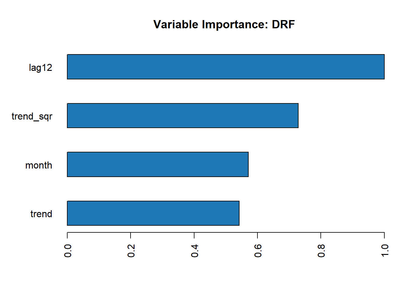
As we can see from the preceding variable importance plot, the lag variable, lag12, is the most important to the model. This shouldn’t be a surprise as we saw the strong relationship between the series and its seasonal lag in the correlation analysis. Right after this, the most important variables are trend_sqr, month, and trend. The output of the model contains (besides the model itself) information about the model’s performance and parameters.
Let’s review the model summary:
rf_md@model$model_summaryModel Summary:
number_of_trees number_of_internal_trees model_size_in_bytes min_depth
1 41 41 31591 8
max_depth mean_depth min_leaves max_leaves mean_leaves
1 12 10.04878 45 66 56.70732We can see that we utilized only 41 trees out of the 500 that were set by the ntrees argument. This is as a result of the stopping parameters that were used on the model. The following plot demonstrates the learning process of the model as a function of the number of trees:
library(plotly)
tree_score <- rf_md@model$scoring_history$training_rmse
plot_ly(x = seq_along(tree_score), y = tree_score,
        type = "scatter", mode = "line") %>%
  layout(title = "The Trained Model Score History",
         yaxis = list(title = "RMSE"),
         xaxis = list(title = "Num. of Trees"))
Last but not least, let’s measure the model’s performance on the testing partition. We will use the h2o.predict function to predict the corresponding values of the series on the testing partition:
# test_h <- as.h2o(test_df)
test_h$pred_rf <- h2o.predict(rf_md, test_h)
h2o.shutdown()
Next, we will transfer the h2o data frame to a data.frame object with the as.data.frame function:
test_1 <- as.data.frame(test_h)Now, we can calculate the MAPE score of the RF model on the test partition:
mape_rf <- mean(abs(test_1$y - test_1$pred_rf) / test_1$y)
mape_rf
[1] 0.04647164As you can see from the model error score, the RF model with its default settings was able to achieve a lower error rate than our benchmark model, that is, the linear regression model, with a MAPE score of 4.6% as opposed to 3.6%.
Generally, when using the default option for the model’s parameters, the model may perform well, but there might be some room left for additional optimization and improvement in regards to the performance of the model. There are a variety of techniques for model optimization and tuning parameters, such as manual tuning, grid search, and algorithm-based tuning.
GRID SEARCH APPROACH
The h2o.grid function allows you to set a set of values for some selected parameters and test their performance on the model in order to identify the tuning parameters that optimize the model’s performance.
Example:
# Start by setting the search parameters
hyper_params_rf <- list(mtries = c(2, 3, 4),
                        sample_rate = c(0.632, 0.8, 0.95),
                        col_sample_rate_per_tree = c(0.5, 0.9, 1.0),
                        max_depth = c(seq(1, 30, 3)),
                        min_rows = c(1, 2, 5, 10))
The more parameters you add or define for a wide range of values, the larger the possible search combination. For efficiency reasons, we will set a random search and restrict the search time to 20 minutes with max_runtime_sec. We will use the same stopping metric that we used previously:
#{r Five}
search_criteria_rf <- list(strategy = "RandomDiscrete",
                           stopping_metric = "rmse",
                           stopping_tolerance = 0.0001,
                           stopping_rounds = 10,
                           max_runtime_secs = 60 * 5)
After we set the search arguments for the h2o.grid function, we can start the search:
#{r Six}
rf2 <- h2o.grid(algorithm = "randomForest",
                search_criteria = search_criteria_rf,
                hyper_params = hyper_params_rf,
                x = x,
                y = y,
                training_frame = train_h,
                ntrees = 5000,
                nfolds = 5,
                grid_id = "rf_grid",
                parallelism = 1,
                seed = 1234)
Note that setting a large number of trees with a tree-based model such as RF or GBM, along with a stopping metric, will ensure that the model will keep building additional trees until it meets the stopping criteria. Therefore, setting the stopping criteria plays a critical roll in both the efficiency of the model and its results.
We will now extract the grid results, sort the models by their RMSE score, and pull the lead model:
rf2_grid_search <- h2o.getGrid(grid_id = "rf_grid",
                               sort_by = "rmse",
                               decreasing = FALSE)
rf_grid_model <- h2o.getModel(rf2_grid_search@model_ids[[1]])
Let’s test the model on the testing partition and evaluate its performance:
test_h$rf_grid <- h2o.predict(rf_grid_model, test_h)
mape_rf2 <- mean(abs(test_1$y - test_1$rf_grid) / test_1$y)
mape_rf2
The additional optimization step contributed to the lift in the model’s accuracy, with a MAPE score of 3.33% compared to 3.7% and 4% for the first RF model we trained, and the linear regression model, respectively.
The following plot provides an additional view of the model’s performance:
plot_ly(data = test_1) %>%
  add_lines(x = ~ date, y = ~y, name = "Actual") %>%
  add_lines(x = ~ date, y = ~ yhat, name = "Linear Regression",
            line = list(dash = "dot")) %>%
  add_lines(x = ~ date, y = ~ pred_rf, name = "Random Forest",
            line = list(dash = "dash")) %>%
  add_lines(x = ~ date, y = ~ rf_grid, name = "Random Forest (grid)",
            line = list(dash = "dash")) %>%
  layout(title = "Total Vehicle Sales - Actual vs. Prediction (Random Forest)",
         yaxis = list(title = "Thousands of Units"),
xaxis = list(title = "Month"))The GBM algorithm is another ensemble and tree-based model. It uses the boosting approach in order to train different subsets of the data, and repeats the training of subsets that the model had with a high error rate. This allows the model to learn from past mistakes and improve the predictive power of the model.
The following example demonstrates the use of the h2o.gbm function for training the GBM model with the same input data we used previously:
Example:
gbm_md <- h2o.gbm(training_frame = train_h,
                  nfolds = 5,
                  x = x,
                  y = y,
                  max_depth = 20,
                  distribution = "gaussian",
                  ntrees = 500,
                  learn_rate = 0.1,
                  score_each_iteration = TRUE
)
We can review the rank of the importance of the model’s variables with the h2o.varimp_plot function:
h2o.varimp_plot(gbm_md)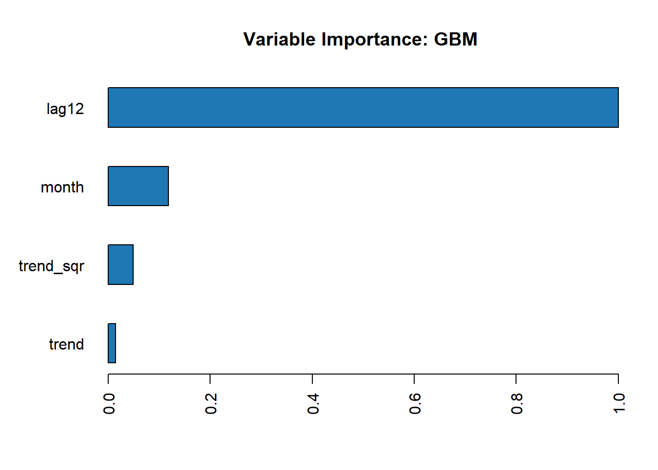
For RF, the GBM model ranks the lag12 variable as the most important to the model. Let’s test the model’s performance on the testing set:
test_h$pred_gbm <- h2o.predict(gbm_md, test_h)
test_1 <- as.data.frame(test_h)
mape_gbm <- mean(abs(test_1$y - test_1$pred_gbm) / test_1$y)
mape_gbm
The GBM model scored the lowest MAPE (is not!) among the models we’ve tested so far with a 3.8% error rate, compared to the RF model (with grid search) and linear regression model. It would be a great exercise to apply a grid search on the GBM model and test whether any additional improvements can be achieved.
Let’s visualize the results and compare the prediction with the actual and baseline prediction:
plot_ly(data = test_1) %>%
  add_lines(x = ~ date, y = ~y, name = "Actual") %>%
  add_lines(x = ~ date, y = ~ yhat,
            name = "Linear Regression",
            line = list(dash = "dot")) %>%
  add_lines(x = ~ date, y = ~ pred_gbm,
            name = "Gradient Boosting Machine", line = list(dash = "dash"))%>%
  layout(title = "Total Vehicle Sales - Actual vs. Prediction (Gradient Boosting Machine)",
         yaxis = list(title = "Thousands of Units"),
xaxis = list(title = "Month"))Let’s take a look at a third approach to tuning ML models. Here, we will use the h2o.automl function that provides an automated approach to training, tuning, and testing multiple ML algorithms before selecting the model that performed best based on the model’s evaluation. It utilizes algorithms such as RF, GBM, DL, and others using different tuning approaches.
Similarly, the h2o.grid function can apply any of the training approaches (CV, training with validation, and so on) during the training process of the models. Let’s use the same input as before, and train the forecasting model:
Example:
autoML1 <- h2o.automl(training_frame = train_h,
                      x = x,
                      y = y,
                      nfolds = 5,
                      max_runtime_secs = 60*20,
                      seed = 1234)
Note that we can set the runtime of the function. A longer running time could potentially yield better results.
In the preceding example, the function’s running time was set to 20 minutes. The function returns a list with the leaderboard of all the tested models:
autoML1@leaderboardNow that we’ve finished the training and testing process of the models, it’s time to finalize the process and choose the model to forecast with the series. We trained the following models:
Baseline model: Linear regression model with 4% MAPE score on the testing partition.
RF: Using default tuning parameters with 3.74% MAPE score on the testing partition.
RF: Using grid search for tuning the model parameters with 3.33% MAPE score on the testing partition.
GBM: Using the default tuning parameters with 2.75% MAPE score on the testing partition.
AutoML: Selecting a deep learning model with 3.48% MAPE score on the testing partition.
Since all of these models achieved better results than the baseline, we can drop the baseline model. Also, since the second RF model (with grid search) achieved better results than the first, there is no point in keeping the first model. This leaves us with three forecasting models, that is, RF (with grid search), GBM, and AutoML. Generally, since the GBM model achieved the best MAPE results, we will select it. However, it is always nice to plot the actual forecast and check what the actual forecast looks like.
Before we plot the results, let’s use these three models to forecast the next 12 months using the data.frame forecast we created in the Forecasting with the Random Forest model and Forecasting with the GBM model sections:
forecast_h$pred_gbm <- h2o.predict(gbm_md, forecast_h)
forecast_h$pred_rf <- h2o.predict(rf_grid_model, forecast_h)
forecast_h$pred_automl <- h2o.predict(autoML1@leader, forecast_h)
We will transform the object back into a data.frame object with the as.data.frame function:
final_forecast <- as.data.frame(forecast_h)Now, we can plot the final forecast with the plotly package:
plot_ly(x = df$date,
        y = df$y,
        type = "scatter",
        mode = "line",
        name = "Actual") %>%
    add_lines(x = final_forecast$date,
              y = final_forecast$pred_rf,
              name = "Random Forest") %>%
    add_lines(x = final_forecast$date,
              y = final_forecast$pred_gbm,
              name = "GBM") %>%
    add_lines(x = final_forecast$date,
              y = final_forecast$pred_automl,
              name = "Auto ML") %>%
    layout(title = "Total Vehicle Sales - Final Forecast",
          yaxis = list(title = "Thousands of Units",
                      range = c(1100, 1750)),
          xaxis = list(title = "Month",
                      range = c(as.Date("2016-01-01"),
                      as.Date("2020-01-01")))
)
It seems that all three models capture the seasonality component of the vehicle sales series. However, it seems that the oscillation of AutoML is higher with respect to one of the RF and GBM models. Therefore, it would make sense to select either the GBM or RF models as the final forecast.
A more conservative approach would be to create and ensemble of the three forecasts by either weighted on regular average. For instance, you can use a simple function for testing the different average of different models and select the combination that minimizes the forecast error rate on the testing set.