library(TSstudio)
data(USVSales)
ts_info(USVSales)
The USVSales series is a ts object with 1 variable and 528 observations
Frequency: 12
Start time: 1976 1
End time: 2019 12 Decomposition of time series data is one of the essential elements of time series analysis, namely, the decomposition process of time series data to its components: the trend, seasonal, and random components.
We will start this analysis by focusing on the moving average (MA) function and see its applications for smoothing time series data, removing seasonality, and estimating a series trend. Once the data has been cleaned and reformatted, one of the first steps of the analysis is to identify the structure of the series components. The decomposition of time series is a generic name for the process of separating a series into its components. This process provides insights into the structural patterns of the series.
Although there are multiple decomposition methods, we will focus on the classical seasonal decomposition method, as most methods are based on a type of extension of this method.
The moving average (MA) is a simple function for smoothing time series data. This function is based on averaging each observation of a series, when applicable, with its surrounding observations, that is, with a past, future, or a combination of both past and future observations, in chronological order.
The output of this transformation process is a smoothed version of the original series.
The main components of the MA function are as follows:
The rolling window: This is a generic function that slides across the series in chronological order to extract sequential subsets
Average function: This is either a simple or weighted average, which is applied on each subset of the rolling window function.
The structure of the rolling window function defines the sub-setting method of series observations, thus playing a pivotal role in the smoothing of time series data process.
The most common types of window structures are as follows:
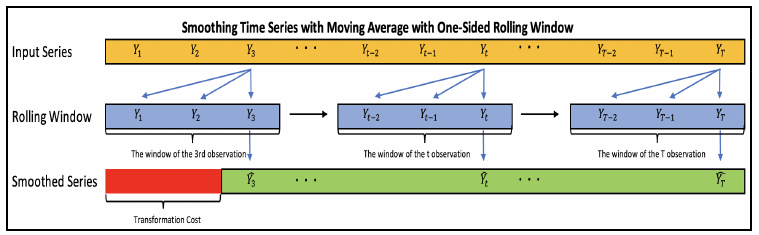
The output of the MA function (marked in green) is missing the first two observations (marked in red), which are considered to be the cost of the transformation process when using a one-sided rolling window.
The window groups each observation with its preceding and leading observations. In this case, you cannot transform the first and last observations of the series (marked in red).
There are two types of averaging methods:
The arithmetic (or simple) average: This is the most common and basic method for averaging a sequence of observations. It is based on summing all the observations and dividing them by the number of observations.
\[\overline{Y} = \frac{\sum_{i=1}^{n}Y_i}{n}\]
The weighted average: This method is based on applying weight to each observation of the series.
\[\overline{Y_t} = {\sum_{i=1}^{n}w_i Y_i}\]
\(w_i\) represents the corresponding weight of the \(i\) observation of \(Y\). A weighted average should be used with time series data when there is a systematic relationship between some observations in the series based on their timestamp distance.
The MA function has a variety of applications, such as data smoothing, noise reduction, and trend estimation. Also, with some small modifications, this function can be used as a forecasting model.
Noise reduction: The use of the MA method creates a smoothing effect that reduces the series variation, smoothing the random noise and outliers.
De-seasonalize: In addition to the noise reduction, MAs can be used to remove the seasonal component (if any). This process has a pivotal role in the classical decomposing process, as it provides an estimation for the trend component, which is then utilized to estimate the seasonal component.
Forecasting: With some small modifications, the MA function can be used to forecast the future observations of the series by averaging the past observations to estimate future values of the series. The averaging method varies from a simple average to more advanced averaging methods.
To calculate different types of MAs we will use the ts_ma function from the TSstudio package, but you can be sure that there is more than one package in R that provides an MA transformation function.
The ts_ma function from the TSstudio package allows us to generate and plot multiple MA outputs simultaneously, using different orders and methods (SMA, two-sided MA, and so on). The main parameters of this function are as follows:
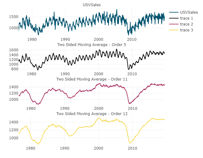
n: This sets the length of the past and future observations to be used in a two-sided MA function. For example, if n is set to three, the window function will group each observation with its past and future three consecutive observations, which will yield a 7 order MA. In addition, it is possible to set this parameter with multiple values in order to generate multiple two-sided MA functions simultaneously using a different order.
n_left/n_right: These are used to customize the MA function by setting the length of the past (n_left) manually and/or the future (n_right) side of the window function. If both parameters are defined, the output is a two-sided MA function, either centered or uncentered. If only one of those parameters is set, the function output is a one-sided MA.
Example:
library(TSstudio)
data(USVSales)
ts_info(USVSales) The USVSales series is a ts object with 1 variable and 528 observations
Frequency: 12
Start time: 1976 1
End time: 2019 12 ts_plot(USVSales,
title = "US MOnthly Total Vehicle Sales",
Ytitle = "Thousands of Units",
Xtitle = "Years",
Xgrid = TRUE,
Ygrid = TRUE)two_sided_ma <- ts_ma(ts.obj = USVSales,
n = c(2,5), # Sets an order 5 and 11 moving average
n_left = 6, n_right = 5, # Sets an order 12 moving average
plot = TRUE,
multiple = TRUE,
margin = 0.04)
Note that the higher the order of the function, the smoother the output. Of course, the smoothing effect comes at the cost of losing observations from both the start and end of the series. The loss of observations is a function of the order of the function, since the higher the order of the MA function, the higher the loss of observations.
The selection of a specific type of MA method depends on the aim of the transformation. Moreover, the use of a different range of order may change the outcome significantly. Generally, when applying both simple and two-sided MAs with arithmetic average using the same order, the output of both methods will be identical but lagged.
The simple moving average (SMA) (one-sided MA) is one of the common MA functions, and, as the name implies, it is also one of the simplest MA functions. This transformation method is based on applying an arithmetic average on a one-sided rolling window. Hence, the rolling window groups each observation in the series (when applicable) with its previous \(n\) consecutive observations in order to calculate their arithmetic average.
The two-sided MA method is based on a two-sided rolling window function, which groups each observation of the series with the past \(n_1\) and future \(n_2\) consecutive observations (as opposed to the SMA or one-sided MA, which use only past \(n-1\) observations). The term two-sided MA refers to the use of the two-sided window function with an arithmetic average.
The output of the two-sided MA function could be either of the following:
Centered: This is when \(n_1\) and \(n_2\) are equal, which ensures that the function output at time t is centered around the t observation of the original y series.
Un-centered: This is when the length of \(n_1\) is different from the length of \(n_2\), or the order of the MA is an even number.
Example:
# Create one-sided and two-sided MA with an order of 12
one_sided_12 <- ts_ma(USVSales,
                      n = NULL,
                      n_left = 11,
                      plot = FALSE)
two_sided_12 <- ts_ma(USVSales,
                      n = NULL,
                      n_left = 6,
                      n_right = 5,
                      plot = FALSE)
one_sided <- one_sided_12$unbalanced_ma_12
two_sided <- two_sided_12$unbalanced_ma_12
We will now bind the output of the one-sided and two-sided MA functions with the USVSales series and plot it with the ts_plot function:
ma <- cbind(USVSales, one_sided, two_sided)
p <- ts_plot(ma,
          Xgrid = TRUE,
          Ygrid = TRUE,
          type = "single",
          title = "One-Sided vs. Two-Sided Moving Average - Order 12")
Next, we will use the layout function from the plotly package to set the plot legend and labels:
library(plotly)
p %>% layout(legend = list(x = 0.05, y = 0.95),
            yaxis = list(title = "Thousands of Units"),
            xaxis = list(title = "Year"))
Conclusion:
It would make sense to use the one-sided MA function when you need to have the most recent observations (as the loss of observations, in this case, is from the beginning of the series).
The use of a centered two-sided MA function (or close to centered when the order of the function is even) is generally more appropriate to apply as a smoother or data filter method. As you can see, the output of the two-sided MA function fits better with the overall changes in the series trend with respect to the one-sided function output. This is mainly due to the fact that there is a delay of five periods between the two methods. This comes at the cost of losing the series’ last 5 observations in addition to the first 6 (as opposed to the last of the first 11 observations of the one-sided function). This makes the use of the two-sided function more expensive when you care about the most recent observations of the series.
Classical decomposition (or classical seasonal decomposition by MA) is one of the most common methods of decomposing a time series down to its components. This method for estimating the three components is based on the use of an MA function followed by simple arithmetic calculations.
This is a three-step process, where each step is dedicated to the estimation of one of the components in sequential order (hence, the calculation of each component is derived from the estimate of the previous component):
Trend estimation: This is the first step of the decomposing process, by using the MA function to remove the seasonal component from the series. The order of the MA function is defined by the frequency of the series. For instance, if the frequency of the input series is monthly (or 12), then the order of the MA should be set to 12. Since we are using a two-sided MA, some of the first and last observations of the trend estimation will be missing.
Seasonal component estimation: A two-step process, starting with de-trending the series by subtracting the trend estimation from the previous step from the series, where:
You can use \(Y_t - {\hat T_t}\) when using the additive model, and \(\frac {Y_t}{\hat T_t}\) when the model is multiplicative. Here, \(Y_t\) is the original series observation at time \(t\) and \(\hat {T_t}\) is the corresponding trend estimation.
After the series is detrended, the next step is to estimate the corresponding seasonal component for each frequency unit (for example, for a monthly series, the seasonal component for January, February, and so on). This calculation is done by grouping the observations by their frequency unit and then averaging each group. The output of this process is a new series with a length that is equal to the series frequency and is ordered accordingly. This series represents the seasonal component of each frequency unit, so this estimation is one-to-many (one estimation for multiple observations).
Irregular component estimation: This is about subtracting the estimation of the trend and seasonal components from the original series. This is \(\hat{I_t} = {Y_t} - \hat{T_t} - \hat{S_t}\) for an additive series, and \(\hat{I_t} = \frac {Y_t}{({\hat T_t} \times {\hat S_t})}\) for a multiplicative series. Here, \(Y_t\) represents the original series at time \(t\), and \(\hat{T_t}\), \(\hat{S_t}\), and \(\hat{I_t}\) represent the corresponding trend and seasonal and irregular components estimate.
The decompose function from the stats package implements this method. By default, this function is set to an additive model.
Example:
data(USVSales)
usv_decompose <- decompose(USVSales)
str(usv_decompose)
List of 6
$ x : Time-Series [1:528] from 1976 to 2020: 885 995 1244 1191 1203 ...
$ seasonal: Time-Series [1:528] from 1976 to 2020: -225.2 -102.4 143 34.5 147.9 ...
$ trend : Time-Series [1:528] from 1976 to 2020: NA NA NA NA NA ...
$ random : Time-Series [1:528] from 1976 to 2020: NA NA NA NA NA ...
$ figure : num [1:12] -225.2 -102.4 143 34.5 147.9 ...
$ type : chr "additive"
- attr(*, "class")= chr "decomposed.ts"class(usv_decompose)[1] "decomposed.ts"From the preceding output you can see that the function returns a list of six objects:
x: This is the original series, a ts object.
seasonal: This is the estimate of the seasonal component, a ts object.
trend: This is the estimate of the series trend, a ts object. You can see that the first (and also the last) observations are missing due to the use of the two-sided MA function. The number of missing values is defined by the order of the MA function.
random: This is the estimate of the irregular component, a ts object. This output is nothing but the remainder of the series and the preceding two components. The random object is missing whenever the trend estimation is missing.
figure: This is the estimated seasonal figure only.
type: This is the type of decomposition, either an additive (the default), or multiplicative model.
Now we can plot the output of the decompose function as plotsupports the decomposed.ts class.
Example:
plot(usv_decompose)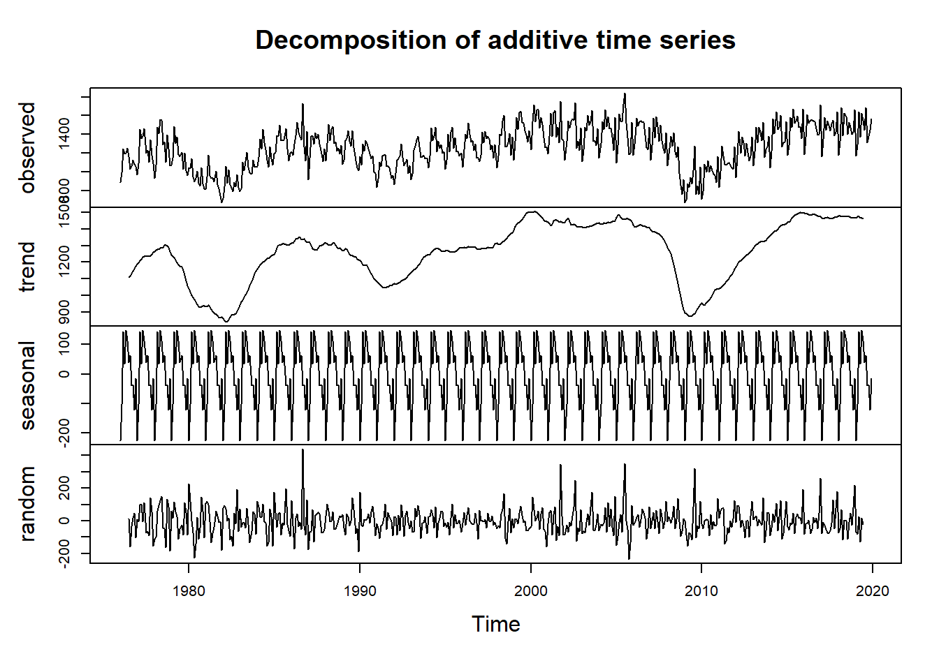
Similarly, if the series has multiplicative growth, like the AirPassengers series, you can set the decomposition process with a multiplicative model:
Example:
air_decompose <- decompose(AirPassengers, type = "multiplicative")
plot(air_decompose)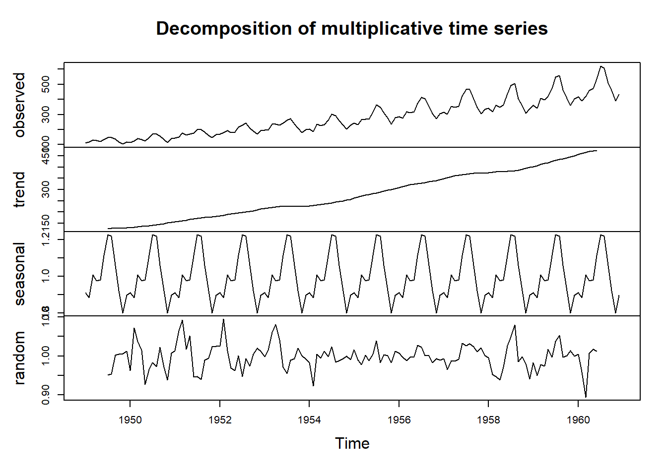
One of the downsides of the classical decomposition method is that seasonal component estimation is based on the arithmetic average, which results in a one-to-many estimation, so there is a single seasonal component estimation for each cycle unit (for example, all observations of the series that occurred in January will have the same seasonal component estimation if the series is monthly). This is not problematic when applying this method to an additive series, such as the US vehicle sales or the monthly natural gas consumption datasets, as the magnitude of the seasonal oscillation remains the same (or close to the same) over time. However, this is not the case for a multiplicative series, as the magnitude of the seasonal oscillation grows over time.