41 Forecasting with ARIMA Models

The Autoregressive Integrated Moving Average (ARIMA) model is the generic name for a family of forecasting models that are based on the Autoregressive (AR) and Moving Average (MA) processes. Among the traditional forecasting models (e.g., linear regression, exponential smoothing, and so on), the ARIMA model is considered as the most advanced and robust approach.

41.1 The Stationary Process

One of the main assumptions of the ARIMA family of models is that the input series follows the stationary process structure. Much of the probability theory of time series is concerned with stationary time series, and for this reason time series analysis often requires one to transform a non-stationary series into a stationary one so as to use this theory. This assumption is based on the Wold representation theorem, which states that any stationary process can be represented as a linear combination of white noise.

Time series data is stationary if the following conditions take place:

The mean and variance of the series do not change over time.
The correlation structure of the series, along with its lags, remains the same over time.

In other words, the properties of one section of the data are much like those of any other section.

The arima.sim function from the stats package enables us to simulate a stationary and non-stationary time series data and plot it with the ts_plot function from the TSstudio package.

The arima.sim function allows us to simulate time series data based on the ARIMA model’s components and main characteristics:

An Autoregressive (AR) process: Establish a relationship between the series and its past $p$ lags with the use of a regression model (between the series and its $p$ lags).
A Moving Average (MA) process: Similar to the AR process, the MA process establishes the relationship with the error term at time $t$ and the past error terms, with the use of regression between the two components (error at time $t$ and the past error terms).
Integrated (I) process: The process of differencing the series with its $d$ lags to transform the series into a stationary state.

Here, the model argument of the function defines $p$, $q$, and $d$, as well as the order of the AR, MA, and I processes of the model.

41.1.1 Stationary series

In the following example, we will simulate an AR process with one lag (that is, $p = 1$) and 500 observations with the arima.sim function. Before running the simulation, we will set the seed value to $12345$:

Example:

set.seed(12345) 
stationary_ts <- arima.sim(model = list(order = c(1,0,0), 
                                        ar = 0.5), 
                           n = 500)

Now let’s plot the simulate time series with the ts_plot function:

Example:

library(TSstudio)
ts_plot(stationary_ts,
        title = "Stationary Time Series",
        Ytitle = "Value",
        Xtitle = "Index")

In this case, overall, the mean of the series, over time, remains around the zero line. In addition, the series’ variance does not change over time.

41.1.2 Non-stationary series

Let’s utilize the arima.sim function to create an example for non-stationary series:

Example:

set.seed(12345)
non_stationary_ts <- arima.sim(model = list(order = c(1,1,0),
                                            ar = 0.3),
                               n = 500)
ts_plot(non_stationary_ts,
        title = "Non-Stationary Time Series",
        Ytitle = "Value",
        Xtitle = "Index")

As you can see this example violates the stationary condition as it is trending over time, which means it is changing over time. Common examples of a series with a non-stationary structure are as follows:

A series with a dominant trend: The series’ mean changes over time as a function of the change in the series trend, and therefore the series is non-stationary.
A series with a multiplicative seasonal component: In this case, the variance of the series is a function of the seasonal oscillation over time, which either increases or decreases over time.

The AirPassenger series (the monthly airline passenger numbers between 1949 and 1960) from the datasets package is a good example of a series that violates the two conditions of the stationary process. Since the series has both a strong linear trend and a multiplicative seasonal component, the mean and variance are both changing over time:

Example:

data(AirPassengers)
ts_plot(AirPassengers,
        title = "Monthly Airline Passenger Numbers 1949-1960",
        Ytitle = "Thousands of Passengers",
        Xtitle = "Year")

41.1.3 Transforming a non-stationary series into a stationary series

In most cases, unless you are very lucky, your raw data would probably come with a trend or other form of oscillation that violates the assumptions of the stationary process. To handle this, you will have to apply some transformation steps in order to bring the series into a stationary state.

Common transformations methods are:

Differencing the series (or de-trending).
Log transformation
or both.

DIFFERENCING TIME SERIES

The most common approach to transforming a non-stationary time series data into a stationary state is by differencing the series with its lags. The main effect of differencing a series is the removal of the series trend (or detrending the series), which help to stabilize the mean of the series.

It is common to use seasonal differencing when a series has a seasonal component. The diff function from the base package differences the input series with a specific lag by setting the lag argument of the function to the relevant lag.

Example:

# First order difference
ts_plot(diff(AirPassengers, lag = 1),
        title = "AirPassengers Series - First Differencing",
        Xtitle = "Year",
        Ytitle = "Differencing of Thousands of Passengers")

You can see that the first difference of the AirPassenger series removed the series trend and that the mean of the series is, overall, constant over time. On the other hand, there is clear evidence that the variation of the series is increasing over time, and therefore the series is not stationary yet.

In addition to the first order difference, taking the seasonal difference of the series could solve this issue. Let’s add the seasonal difference (double differencing) to the first order difference and plot it again:

Example:

ts_plot(diff(diff(AirPassengers, lag = 1), 12),
        title = "AirPassengers Series - First and Seasonal Differencing",
        Xtitle = "Year",
        Ytitle = "Differencing of Thousands of Passengers")

The seasonal difference did a good job of stabilizing the series variation, as the series now seems to be stationary.

LOG TRANSFORMATION

We can utilize the log transformation approach to stabilize a multiplicative seasonal oscillation, if it exists. This approach is not a replacement for differencing, but an addition.

For instance, in the example of the AirPassenger in the preceding section, we saw that the first differencing is doing a great job in stabilizing the mean of the series, but is not sufficient enough to stabilize the variance of the series. Therefore, we can apply a log transformation to transform the seasonal structure from multiplicative to additive and then apply the first-order difference to stationarize the series:

Example:

ts_plot(diff(log(AirPassengers), lag = 1),
    title = "AirPassengers Series - First Differencing with Log
    Transformation",
    Xtitle = "Year",
    Ytitle = "Differencing/Log of Thousands of Passengers")

The log transformation with the first-order differencing is doing a better job of transforming the series into a stationary state with respect to the double differencing (first-order with seasonal differencing) approach we used prior.

41.1.4 The random walk process

The random walk, in the context of time series, describes a stochastic process of an object over time, where the main characteristics of this process are as follows:

The starting point of this process at time $0 - Y_0$ is known
The movement (or the walk) of the series with random walk process from time $t-1$ to time $t$ are defined with the following equation:

$Y_t = Y_t-1 + \epsilon_t$

The following example demonstrates the simulation of 20 different random walk paths of 500 steps, all starting at point 0 at time 0. We will create two plots: one for the random walk paths and another for their first-order difference.

Example:

library(plotly)
set.seed(12345)
p1 <- plot_ly()
p2 <- plot_ly()
for(i in 1:20){
  rm <- NULL
  rw <- arima.sim(model = list(order = c(0, 1, 0)), n = 500)
  p1 <- p1 %>% add_lines(x = time(rw), y = as.numeric(rw))
  p2 <- p2 %>% add_lines(x = time(diff(rw)), y = as.numeric(diff(rw)))
  }

Here, $p1$ represents the plot of the random walk simulation:

p1 %>% layout(title = "Simulate Random Walk",
              yaxis = list(title = "Value"),
              xaxis = list(title = "Index")) %>%
  hide_legend()

Here, $p2$ represents the corresponding plot of the first-order differencing of the random walk simulation:

p2 %>% layout(title = "Simulate Random Walk with First-Order Differencing",
              yaxis = list(title = "Value"),
              xaxis = list(title = "Index")) %>%
  hide_legend()

41.2 The AR Process

The $AR$ process defines the current value of the series, $Y_t$, as a linear combination of the previous $p$ lags of the series, and can be formalized with the following equation:

\[AR(p): Y_t = c + \sum^{p}_{i=1} \phi_i Y_{t-i} + \epsilon_t\]

Where:

$AR(p)$ is the notation for an $AR$ process with p-order.
$c$ represents a constant (or drift).
$p$ defines the number of lags to regress against $Y_t$.
$\phi_i$ is the coefficient of the $i$ lag of the series (here, must be between -1 and 1, otherwise, the series would be trending up or down and therefore cannot be stationary over time).
$Y_{t-i}$ is the $i$ lag of the series.
$\epsilon_t$ represents the error term, which is white noise.

An AR process can be used on time series data if, and only if, the series is stationary. Therefore, before applying an $AR$ process on a series, you will have to verify that the series is stationary. Otherwise, you will have to apply some transformation method (such as differencing, log transformation, and so on) to transform the series into a stationary state.

41.2.1 Example of AR process

Task	Function	Variable
Simulate and plot a AR(2) series	`arima.sim` `ts_plot`	`ar2`
Model (fit) a AR(2)	`ar(ar2)`	`md_ar`
Identify the AR(2) process - `acf` output tails off and `pacf`cuts off at lag $p$	`acf(ar2)` `pacf(ar2)`	N/A
Forecast	`forecast(md_ar)`	`ar_fc`

In the following example, we will utilize the arima.sim function again to simulate an $AR(2)$ process structure time series data with 500 observations, and then use it to fit an $AR$ model. We will use the model argument to set the $AR$ order to $2$ and set the lags coefficients $\phi_1 = 0.9$ and $\phi_2 = -0.3$:

Example:

set.seed(12345)
ar2 <- arima.sim(model = list(order = c(2,0,0),
                              ar = c(0.9, -0.3)),
                 n = 500)

Let’s review the simulate time series:

ts_plot(ar2,
        title = "Simulate AR(2) Series",
        Ytitle = "Value",
        Xtitle = "Index")

The ar function from the stats package allows us to fit an $AR$ model on time series data and then forecast its future values. This function identifies the $AR$ order automatically based on the Akaike Information Criterion (AIC). The method argument allows you to define the coefficients estimation method, such as the ordinary least squares (OLS), maximum likelihood estimation (MLE), and Yule-Walker (default).

Let’s apply the ar function to identify the $AR$ order and estimate its coefficients accordingly:

Example:

md_ar <- ar(ar2)
md_ar


Call:
ar(x = ar2)

Coefficients:
      1        2  
 0.8851  -0.2900  

Order selected 2  sigma^2 estimated as  1.049

As you can see the ar function was able to identify that the input series is a second order AR process, and provided a fairly close estimate for the value of the actual coefficients, $\hat\phi_1 = 0.88$, $\hat\phi_2 = -0.29$ (as opposed to the actual coefficients’ values, $\phi_1 = 0.9$, $\phi_2 = -0.3$).

Forecast the AR model

The following code demonstrates the forecast of the next 100 observations of the $AR$ model we trained previously with the ar function:

Example:

library(forecast)
ar_fc <- forecast(md_ar, h = 100)
# Use `plot_forecast to plot the forecast output:
plot_forecast(ar_fc,
              title = "Forecast AR(2) Model",
              Ytitle = "Value",
              Xtitle = "Year")

41.2.2 Identifying the AR process and its characteristics

In the preceding example, we simulated an $AR(2)$ series, and it was clear that we need to apply an $AR$ model on the data. However, when working with real-time series data, you will have to identify the structure of the series before modeling it.

In the world of the non-seasonal ARIMA family of models, a series could have one of the following structures:

$AR$.
$MA$.
Random walk.
A combination of the preceding three (for example, $AR$ and $MA$ processes).

Identifying the series structure includes the following two steps:

Categorizing the type of process (for example, $AR$, $MA$, and so on).
Once we have classified the process type, we need to identify the order of the process (for example, $AR(1)$, $AR(2)$, and so on).

Utilizing the autocorrelation function (ACF) and partial autocorrelation function (PACF), allows us to classify the process type and identify its order.

If the ACF output tails off and the PACF output cuts off at lag $p$, this indicates that the series is an $AR(p)$ process.

Example:

# Use the `par` function to plot the two plots side by side
par(mfrow=c(1,2))
# Generate the plots with the acf and pacf functions
acf(ar2)
pacf(ar2)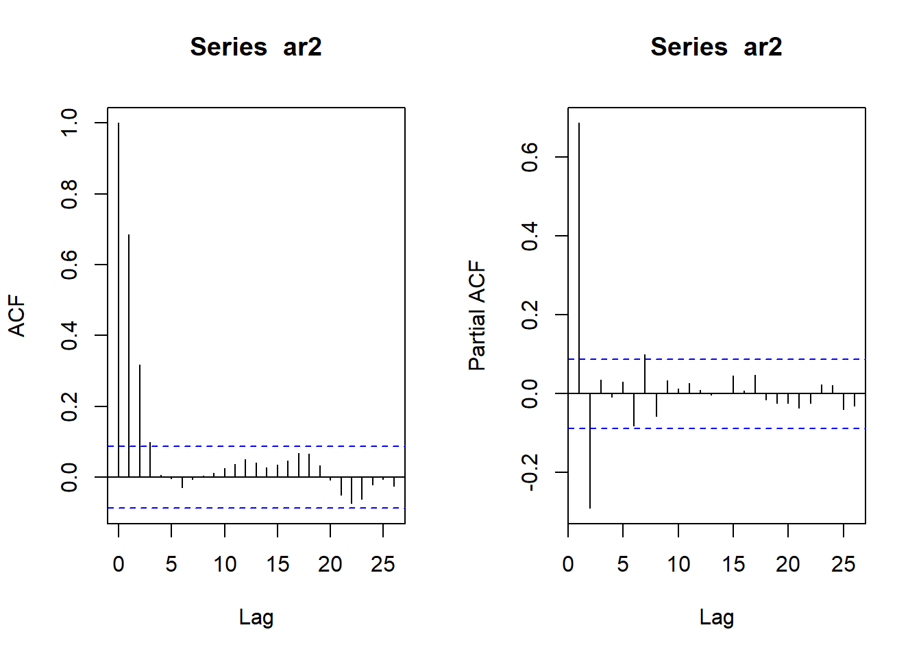

In the case of the ar2 series, you can see that the ACF plot is tailing off and that the PACF plot is cut off at the second lag. Therefore, we can conclude that the series has a second order AR process.

41.3 The MA Process

In some cases, the forecasting model is unable to capture all the series patterns, and therefore some information is left over in model residuals (or forecasting error). The goal of the moving average process is to capture patterns in the residuals, if they exist, by modeling the relationship between $Y_t$, the error term, $\epsilon_t$, and the past $q$ error terms of the models (for example, $\epsilon_{t-1}$, $\epsilon_{t-2}$, $\epsilon_{t-q}$).

The structure of the MA process is fairly similar to the ones of the $AR$. The following equation defines an $MA$ process with a $q$ order:

\[MA(q): Y_t = \mu + \epsilon_t + \sum^{q}_{i=1} \theta_i \epsilon_{t-i}\] Where:

$MA(q)$ is the notation for an $MA$ process with q-order.
$\mu$ represents the mean of the series.
$\epsilon_{t-q}$,…, $\epsilon_t$ are white noise error terms.
$\theta_i$ is the corresponding coefficient of $\epsilon_{t-i}$
$q$ defines the number of past error terms to be used in the equation.

Like the $AR$ process, the MA equation holds only if the series is a stationary process; otherwise, a transformation must be used on the series before applying the $MA$ process.

41.3.1 Example of MA process

Task	Function	Variable
Simulate and plot a MA(2) series	`arima.sim` `ts_plot`	`ma2`
Model (fit) a MA(2)	`arima`	`md_ma`
Identify the MA process - `acf`is cut off at lag $q$ and `pacf` tails off	`acf(ma2)` `ccf(ma2)`	N/A
Forecast the MA model	`forecast(md_ma)`	`ma_fc`

We will utilize the arima.sim function to simulate a series with an $MA(2)$ structure. In this case, we will set the $q$ parameter in the order argument to $2$ and set the $MA$ coefficients to $0.5$ and $-0.3$:

Example:

set.seed(12345)
ma2 <- arima.sim(model = list(order = c(0, 0, 2),
                              ma = c(0.5, -0.3)),
                 n = 500)
# Use the ts_plot function to plot the simulated series
ts_plot(ma2,
        title = "Simulate MA(2) Series",
        Ytitle = "Value",
        Xtitle = "Index")

Modeling the MA process can be done with the arima function from the stats package. This function, when setting the order of the $AR$ and the differencing components of the model to $0$ with the order argument (that is, $p = 0$ and $d = 0$), is modeling only on the MA component.

Example:

# Apply a second-order MA model with the arima function
# on the simulated MA(2) series
md_ma <- arima(ma2, order = c(0,0,2), method = "ML")

Similar to the ar function, you can select the coefficients estimation approach. In this case, there are three methods: maximum likelihood (ML), minimize conditional sum-of-squares (CSS), and the combination of the two, which is known as CSS-ML.

The output of the arima function is more detailed than the ones of the ar function, as it also provides the level of significance of each coefficient (the s.e.):

md_ma


Call:
arima(x = ma2, order = c(0, 0, 2), method = "ML")

Coefficients:
        ma1      ma2  intercept
      0.530  -0.3454     0.0875
s.e.  0.041   0.0406     0.0525

sigma^2 estimated as 0.9829:  log likelihood = -705.81,  aic = 1419.62

41.3.2 Identifying the MA process and its characteristics

Similar to the $AR4 process, we can identify an MA process and its order with the $ACF$ and $PACF$ functions. If the ACF is cut off at lag $q$ and the PACF function tails off, we can conclude that the process is an $MA(q)$. Let’s repeat the process we applied on the ar2 series with the ma2 series:

Example:

par(mfrow=c(1,2))
acf(ma2)
pacf(ma2)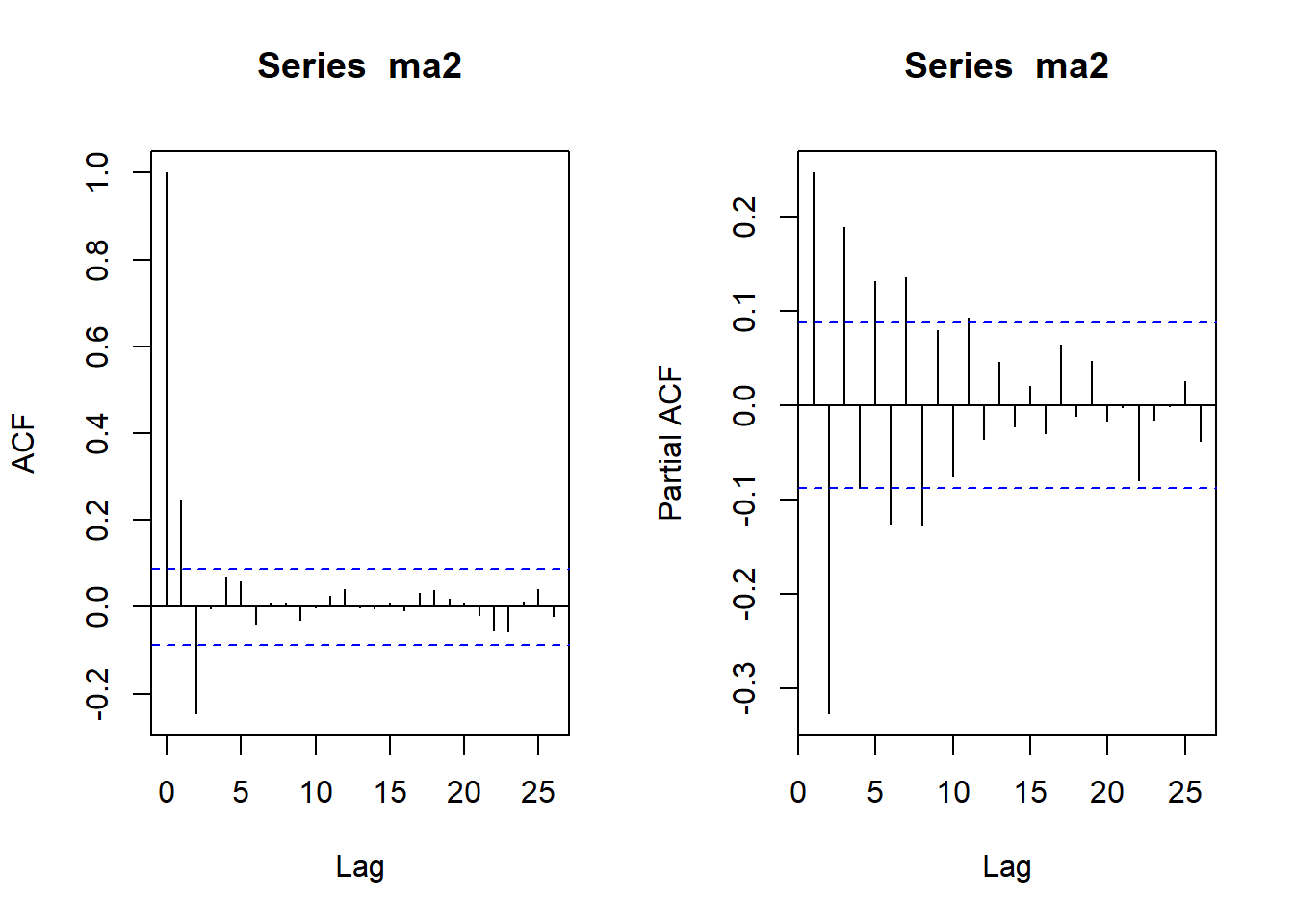

In the case of the ma2 series, the $ACF$ plot is cut off on the second lag (note that lag $0$ is the correlation of the series with itself, and therefore it is equal to $1$ and we can ignore it), and so the $PACF$ tails off. Therefore, we can conclude that the ma2 series is an $MA(2)$ process.

41.4 The ARMA model

Up until now, we have seen how the applications of $AR$ and $MA$ are processed separately. However, in some cases, combining the two allows us to handle more complex time series data. The ARMA model is a combination of the $AR(p)$ and $MA(q)$ processes and can be written as follows:

\[ARMA(p,q): Y_t = c + \sum^{p}_{i=1} \phi_i Y_{t-i} + \sum^{q}_{i=1} \theta_i \epsilon_{t-i} + \epsilon_t\] For instance, an ARMA(3,2) model is defined by the following equation:

\[Y_t = c + \phi_1 Y_{t-i} + \phi_2 Y_{t-2} + \phi_3 Y_{t-3} + \theta_1 \epsilon_{t-1} + \theta_2 \epsilon_{t-2} + \epsilon_t\]

41.4.1 Example of ARMA process

Task	Function	Variable
Simulate and plot a ARMA(1,2) series	`arima.sim`	`arma`
Model (fit) a ARMA(1,2)	`arima`	`arma.md`
Identify the ARMA process - `acf`is cut off at lag $q$ and `pacf` tails offIdentify the MA process - both `acf` and `pacf` tails off	`acf` `ccf`	N/A
Forecast the ARMA model	`forecast(arma.md)`	`arma_fc`

Let’s simulate a time series data with an ARMA(1,2) structure with the arima.sim function and review the characteristics of the $ARMA$ model. We will set the $p$ and $q$ parameters of the order argument to $1$ and $2$, respectively, and set the $AR$ coefficient as $0.7$, and the $MA$ coefficients as $0.5$ and $-0.3$:

Example:

set.seed(12345)
arma <- arima.sim(model = list(order(1,0,2),
                               ar = c(0.7),
                               ma = c(0.5,-0.3)),
                  n = 500)
# Plot and review the series structure
ts_plot(arma,
        title = "Simulate ARMA(1,2) Series",
        Ytitle = "Value",
        Xtitle = "Index")

Fitting an ARMA model is straightforward with the arima function. In this case, we have to set the $p$ and $q$ parameters on the order argument:

arma_md <- arima(arma, order = c(1,0,2))
arma_md


Call:
arima(x = arma, order = c(1, 0, 2))

Coefficients:
         ar1     ma1      ma2  intercept
      0.7439  0.4785  -0.3954     0.2853
s.e.  0.0657  0.0878   0.0849     0.1891

sigma^2 estimated as 1.01:  log likelihood = -713.18,  aic = 1436.36

You can observe from the following output of the fitted model that the values of the model coefficients are fairly close to the one we simulated.

Here, as the coefficient’s name implies, ar1, ma1, and ma2 represent the estimation of the $\phi_1$, $\theta_1$, and $\theta_2$ coefficients, respectively. You can note that the intercept parameter is not statistically significant, which should make sense as we didn’t add an intercept to the simulated data.

41.4.2 Identifying an ARMA process

Identifying the $ARMA$ process follows the same approach that we used previously with the $AR$ and $MA$ processes. An ARMA process exists in time series data if both the ACF and PACF plots tail off, as we can see in the following example:

Example:

par(mfrow=c(1,2))
acf(arma)
pacf(arma)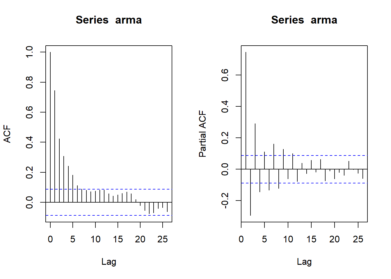

On the other hand, unlike the $AR$ and $MA$ processes, we cannot conclude the order of the ARMA process. There are several approaches for tuning the ARMA $p$ and $q$ parameters:

Manual tuning: By starting with a combination of $p$ and $q$ and using some error criteria for identifying the model parameters.
Grid search: By trying different combinations of the $p$ and $q$ parameters based on the grid matrix. Likewise, manual tuning and the selection of a specific combination of $p$ and $q$ parameters should be based on error criterion.
Algorithm-based search: By using a function or algorithm for tuning the model parameters.

41.5 The ARIMA model

One of the limitations of the $AR$, $MA$, and $ARMA$ models is that they cannot handle non-stationary time series data. Therefore, if the input series is non-stationary, a pre-processing step is required to transform the series from a non-stationary state into a stationary state.

The ARIMA model provides a solution for this issue by adding the integrated process for the $ARMA$ model. The Integrated (I) process is simply differencing the series with its lags, where the degree of the differencing is represented by the $d$ parameter.

The differencing process is one of the ways you can transform the methods of a series from non-stationary to stationary. For instance, $Y_t - Y_{t-1}$ represents the first differencing of the series, while $(Y_t - Y_{t-1}) - (Y_{t-1} - Y_{t-2})$ represents the second differencing.

We can generalize the differencing process with the following equation:

\[Y_d = (Y_t - Y_{t-1}) - ... - (Y_{t-d+1} - Y_{t-d})\]

Where, $Y_d$ is the $d$ differencing of the series.

Let’s add the differencing component to the $ARMA$ model and formalize the $ARIMA(p,d,q)$ process with a p-order $AR$ process, d-degree of differencing, and q-order $MA$ process:

\[ARIMA(p,q,d): Y_d = c + \sum^{p}_{i=1} \phi_i Y_{d-i} + \sum^{q}_{i=1} \theta_i \epsilon_{t-i} + \epsilon_t\]

Note that both the $AR$ and $MA$ models can be represented with the $ARMA$ model, and that you can also represent the $AR$, $MA$, or $ARMA$ models with the $ARIMA$ model, for example:

The ARIMA(0, 0, 0) model is equivalent to white noise.
The ARIMA(0, 1, 0) model is equivalent to a random walk.
The ARIMA(1, 0, 0) model is equivalent to an AR(1) process.
The ARIMA(0, 0, 1) model is equivalent to an MA(1) process.
The ARIMA(1, 0, 1) model is equivalent to an ARMA(1,1) process.

41.5.1 Identifying an ARIMA process

Identifying and setting the $ARIMA model$ is a two-step process based on the following steps:

Identify the degree of differencing that is required to transfer the series into a stationary state.
Identify the ARMA process (or AR and MA processes), as introduced in the previous section.

Based on the findings of these steps, we will set the model parameters $p$, $d$, and $q$.

Similar to the setting the $d$ parameter (the degree of differencing of the series) can be done with the ACF and PACF plots. In the following example, we will use the monthly prices of Robusta coffee since 2000.

41.5.2 Example of ARIMA process

Task	Function	Variable
Plot the series	`ts_plot (robusta_price)`	`robusta_price`
Identify the relationship between the series and its lags	`acf(robusta_price)`	N/A
First differencing the series	`diff(robusta_price)`	`robusta_price_d1`
Determine the order of the model	`acf(robusta_price_d1) pacf(robusta_price_d1)`	N/A
Fit the model ARIMA	`arima(robusta_price)`	`robusta_md`
Check the residuals	`checkresiduals(robusta_md)`

We first start the $ARIMA$ process by extracting the data set and visually analyzing its structure with a plot of the series.

Example:

data("Coffee_Prices")
robusta_price <- window(Coffee_Prices[,1], start = c(2000, 1))
ts_plot(robusta_price,
        title = "The Robusta Coffee Monthly Prices",
        Ytitle = "Price in USD",
        Xtitle = "Year")

As you can see, the $Robusta$ coffee prices over time are trending up, and therefore it is not in a stationary state. In addition, since this series represents continues prices, it is likely that the series has a strong correlation relationship with its past lags (as changes in price are typically close to the previous price).

# Identify the type of relationship between the series and it lags
acf(robusta_price)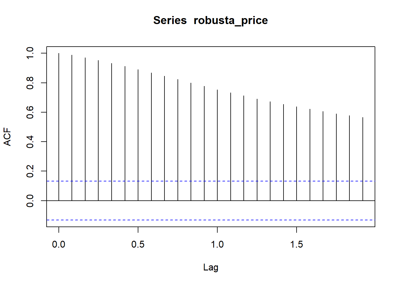

As you can see in the preceding output of the ACF plot, the correlation of the series with its lags is slowly decaying over time in a linear manner. Removing both the series trend and correlation between the series and its lags can be done by differencing the series.

# We will start with the first differencing using the diff function
robusta_price_d1 <- diff(robusta_price)

Let’s review the first difference of the series with the acf and pacf functions:

par(mfrow=c(1,2))
acf(robusta_price_d1)
pacf(robusta_price_d1)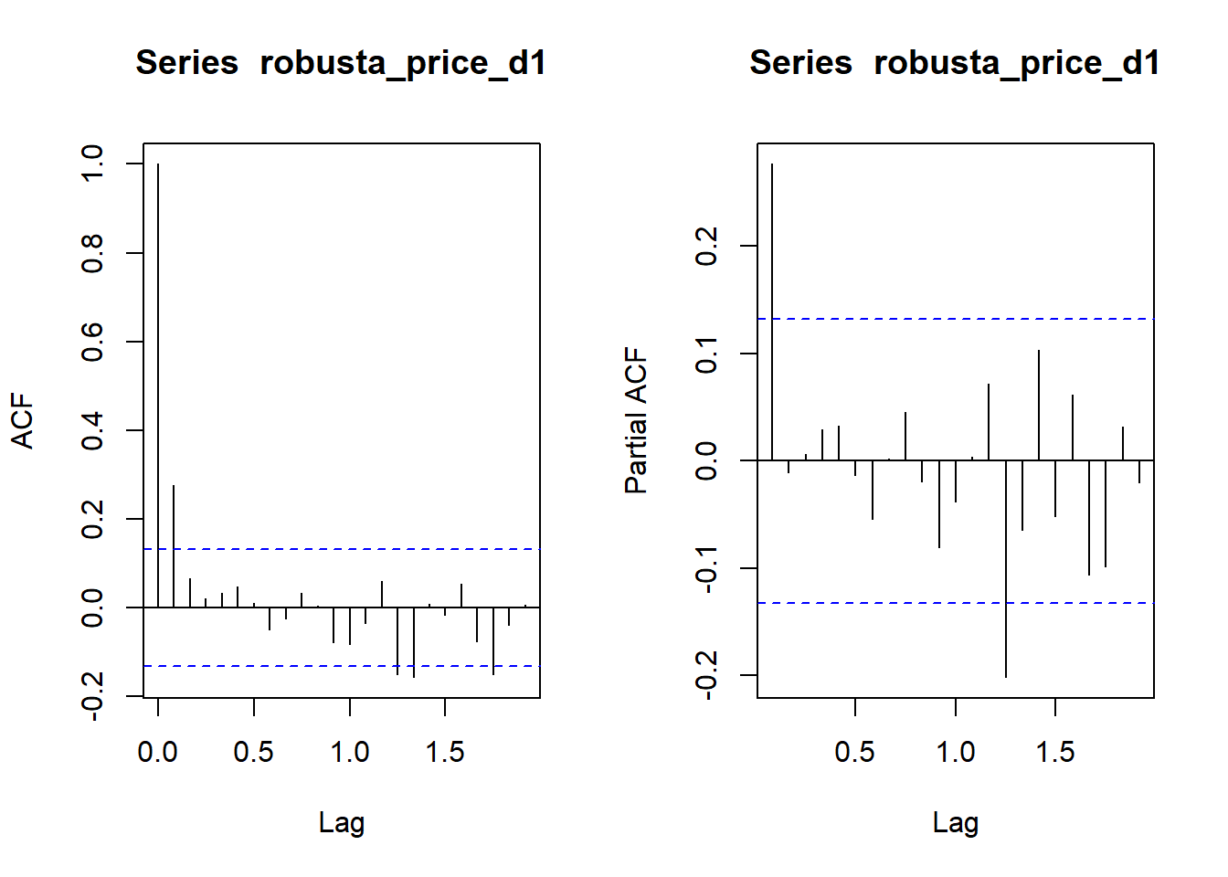

The $ACF$ and $PACF$ plots of the first difference of the series indicate that an $AR(1)$ process is appropriate to use on the differenced series since the $ACF$ is tailing off and the PACF cuts on the first lag. Therefore, we will apply an $ARIMA(1,1,0)$ model on the robusta_price series to include the first difference:

robusta_md <- arima(robusta_price, order = c(1, 1, 0))
# Use the summary function to review the model details
summary(robusta_md)


Call:
arima(x = robusta_price, order = c(1, 1, 0))

Coefficients:
         ar1
      0.2780
s.e.  0.0647

sigma^2 estimated as 0.007142:  log likelihood = 231.38,  aic = -458.76

Training set error measures:
                      ME       RMSE        MAE        MPE     MAPE     MASE
Training set 0.002595604 0.08432096 0.06494772 0.08104715 4.254984 1.001542
                    ACF1
Training set 0.001526295

You can see from the model summary output that the ar1 coefficient is statistically significant. Last but not least, we will check the model residuals:

checkresiduals(robusta_md)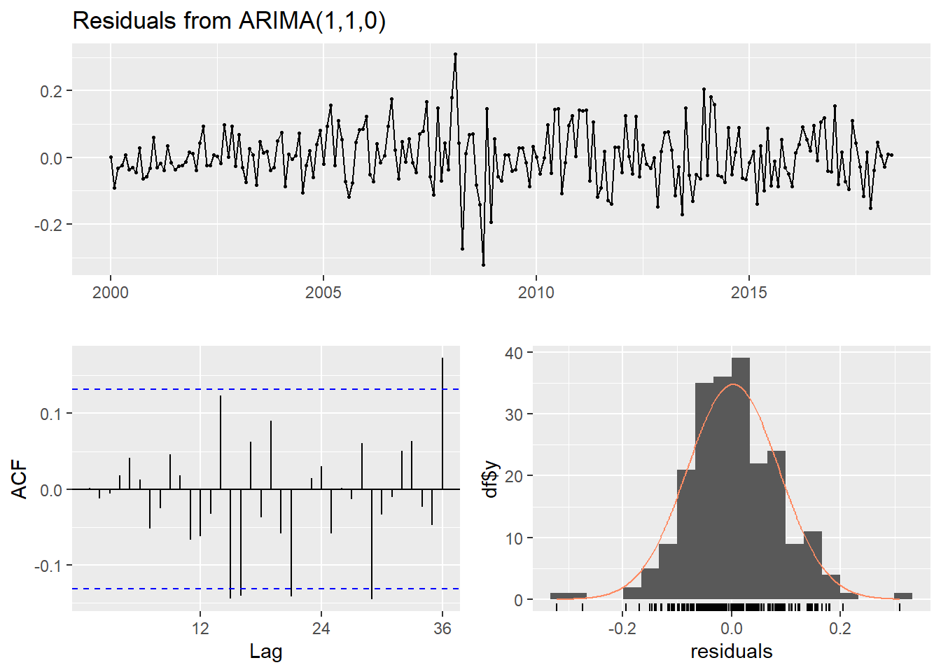


    Ljung-Box test

data:  Residuals from ARIMA(1,1,0)
Q* = 26.896, df = 23, p-value = 0.2604

Model df: 1.   Total lags used: 24

Overall, the plot of the model’s residuals and the Ljung-Box test indicate that the residuals are white noise. The $ACF$ plot indicates that there are some correlated lags, but they are only on the border of being significant and so we can ignore them.

41.6 The Seasonal ARIMA Model (SARIMA)

The Seasonal ARIMA (SARIMA) model is a version of the $ARIMA$ model for time series with a seasonal component. Recall that a time series with a seasonal component has a strong relationship with its seasonal lags. The $SARIMA$ model is utilizing the seasonal lags in a similar manner to how the $ARIMA$ model is utilizing the non-seasonal lags with the $AR$ and $MA$ processes and differencing. It does this by adding the following three components to the $ARIMA$ model:

SAR(P) process: A seasonal $AR$ process of the series with its past $P$ seasonal lags. For example, a $SAR(2)$ is an $AR$ process of the series with its past two seasonal lags, that is, $Y_t = c + \Phi_1 Y_{t-f} + \Phi_2 Y_{t-2f} + \epsilon_t$ , where $\Phi$ represents the seasonal coefficient of the SAR process, and $f$ represents the series frequency.
SMA(Q) process: A seasonal $MA$ process of the series with its past $Q$ seasonal error terms. For instance, a $SMA(1)$ is a moving average process of the series with its past seasonal error term, that is, $Y_t = \mu + \epsilon_t + \Theta_1 \epsilon_{t-f}$, where $\Theta$ represents the seasonal coefficient of the SMA process, and $f$ represents the series frequency.
SI(D) process: A seasonal differencing of the series with its past $D$ seasonal lags. In a similar manner, we can difference the series with its seasonal lag, that is, $Y_{D=1} = Y_t - Y_{t-f}$.

We use the following notation to denote the SARIMA parameters:

\[SARIMA(p,d,q) \times (P,D,Q)_s\]

The $p$ and $q$ parameters define the order of the $AR$ and $MA$ processes with its non-seasonal lags, respectively, and $d$ defines the degree of differencing of the series with its non-seasonal lags. Likewise, the $P$ and $Q$ parameters represent the corresponding order of the seasonal $AR$ and $MA$ processes of the series with its seasonal lags, and $D$ defines the degree of differencing of the series with its non-seasonal lags. For example, a $SARIMA(1,0,0) \times (1,1,0)_s$ model is a combination of an $AR$ process of one non-seasonal and one seasonal lag, along with seasonal differencing.

41.6.1 Forecasting US monthly natural gas consumption with the SARIMA model

We will forecast the monthly consumption of natural gas in the US using the $SARIMA$ model. Let’s load the $USgas$ series from the TSstudio package:

Task	Function	Variable
Plot the series	`ts_plot(USgas)`
Split the series into training and testing partitions	`ts_split(USgas, sample.out = 12)`	`train` `test`
Diagnose the series correlation with its seasonal lags	`acf(train, lag.max = 60)` `pacf(train, lag.max = 60)`	N/A
Conduct a seasonal differencing of the series and plot the output and check if in stationary state	`diff(train, 12)` `ts_plot(USgas)`	`USgas_d12`
Add the first differencing of the series	`diff(diff(USgas_d12, 1)) ts_plot(USgas_d12_1)`	`USgas_d12_1`
Review the `ACF` and `PACF` functions again to identify the required process	`acf(USgas_d12_1)` `ccf(USgas_d12_1)`	N/A

We will first start plotting the $USgas$ series and reviewing its main characteristics.

Example:

data(USgas)
# Plot the series and review its main characteristics
ts_plot(USgas,
        title = "US Monthly Natural Gas consumption",
        Ytitle = "Billion Cubic Feet",
        Xtitle = "Year")

The USgas series has a strong seasonal pattern, and therefore among the $ARIMA$ family of models, the $SARIMA$ model is the most appropriate model to use. In addition, since the series is trending up, we can already conclude that the series is not stationary and some differencing of the series is required.

We will start by setting the training and testing partitions with the ts_split functions, leaving the last 12 months of the series as the testing partition:

USgas_split <- ts_split(USgas, sample.out = 12)
train <- USgas_split$train
test <- USgas_split$test

We will conduct diagnostics in regards to the series correlation with the ACF and PACF functions. Since we are interested in viewing the relationship of the series with its seasonal lags, we will increase the number of lags to calculate and display by setting the lag.max argument to $60$ lags:

par(mfrow=c(1,2))
acf(train, lag.max = 60)
pacf(train, lag.max = 60)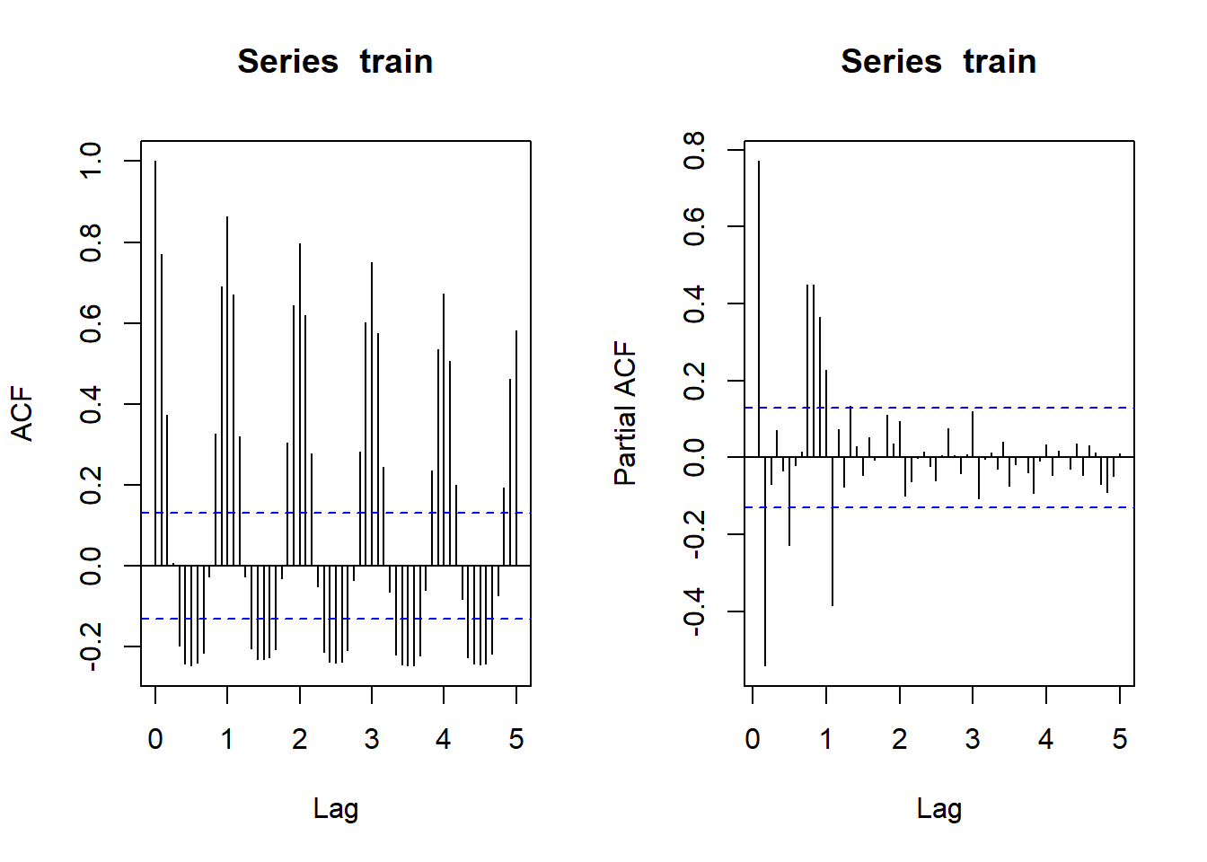

The preceding ACF plot indicates that the series has a strong correlation with both the seasonal and non-seasonal lags. Furthermore, the linear decay of the seasonal lags indicates that the series is not stationary and that seasonal differencing is required.

We will start with a seasonal differencing of the series and plot the output to identify whether the series is in a stationary state:

USgas_d12 <- diff(train, 12)
ts_plot(USgas_d12,
      title = "US Monthly Natural Gas consumption - First Seasonal Difference",
      Ytitle = "Billion Cubic Feet (First Difference)",
      Xtitle = "Year")

While we removed the series trend, the variation of the series is not stable yet. Therefore, we will also try to take the first difference of the series:

USgas_d12_1 <- diff(diff(USgas_d12, 1))
ts_plot(USgas_d12_1,
      title = "US Monthly Natural Gas consumption - First Seasonal and Non-Seasonal Differencing",
      Ytitle = "Billion Cubic Feet (Difference)",
      Xtitle = "Year")

After taking the first order differencing, along with the first order seasonal differencing, the series seems to stabilize around the zero $x$ axis line (or fairly close to being stable). After transforming the series into a stationary state, we can review the ACF and PACF functions again to identify the required process:

par(mfrow=c(1,2))
acf(USgas_d12_1, lag.max = 60)
pacf(USgas_d12_1, lag.max = 60)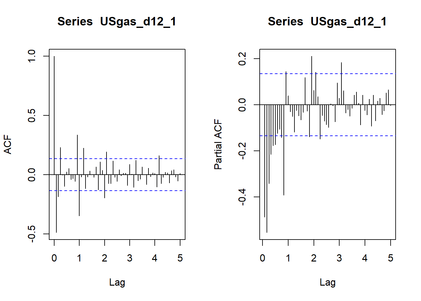

The main observation from the preceding $ACF$ and $PACF$ plots is that both the non-seasonal and seasonal lags (in both plots) are tailing off. Hence, we can conclude that after we difference the series and transform them into a stationary state, we should apply an ARMA process for both the seasonal and non-seasonal components of the SARIMA model.

TUNING PROCESS

The tuning process of the $SARIMA$ model parameters follow the same steps that we applied previously with the $ARMA$ model:

We set the model maximum order (that is, the sum of the six parameters of the model).
We set a range of a possible combination of the parameters’ values under the model’s maximum order constraint.
We test and score each model, that is, a typical score methodology with the AIC (which we used previously) or BIC.
We select a set of parameter combinations that give the best results.

Now, we will start the tuning process for the USgas series by setting the model order to seven and setting the values of the model parameters to be in the range of $0$ and $2$. Given that we already identified the values of $d$ and $D$ (for example, $d = 1$ and $D = 1$), which are the differencing parameters of the SARIMA model, we now can focus on tuning the remaining four parameters of the model, that is, $p$, $q$, $P$, and $Q$. Let’s define those parameters and assign the search values:

p <- q <- P <- Q <- 0:2

Under the model’s order constraint and the possible range of values of the model parameters, there are 66 possible combinations. Therefore, it will make sense, in this case, to automate the search process and build a grid search function to identify the values of the parameters that minimize the AIC score.

We will utilize the expand.grid function in order to create a data.frame with all the possible search combinations:

arima_grid <- expand.grid(p,q,P,Q)
names(arima_grid) <- c("p", "q", "P", "Q")
arima_grid$d <- 1
arima_grid$D <- 1

Next, we will trim the grid search table by using combinations that exceed the order constraint of the model (for example, $k \le 7$). We will calculate and assign this to the $k$ variable with the rowSums function:

arima_grid$k <- rowSums(arima_grid)

We will utilize the filter function from the dplyr package to remove combinations where the k value is greater than $7$:

library(dplyr)
arima_grid <- arima_grid %>% filter(k <= 7)

Now that the grid search table is ready, we can start the search process. We will use the lapply function to iterate over the grid search table. This function will train the SARIMA model and score its AIC for each set of parameters in the grid search table. The arima function can train the SARIMA model by setting the seasonal argument of the model with the values of $P$, $D$, and $Q$:

arima_search <- lapply(1:nrow(arima_grid), function(i){
  md <- NULL
  md <- arima(train, order = c(arima_grid$p[i], 1, arima_grid$q[i]), seasonal = list(order = c(arima_grid$P[i], 1, arima_grid$Q[i])))
  results <- data.frame(p = arima_grid$p[i], d = 1, q = arima_grid$q[i],
                        P = arima_grid$P[i], D = 1, Q = arima_grid$Q[i],
                        AIC = md$aic)
}) %>% bind_rows() %>% arrange(AIC)

We used the bind_rows and arrange functions to append the search results and arranged the table for the dplyr functions. Let’s review the top results of the search table:

head(arima_search)

The leading model based on the preceding search table is the model $SARIMA(1,1,1)(2,1,1)_{12}$. Before we finalize the forecast, let’s evaluate the selected model’s performance on the testing set.

We will retrain the model using the settings of the selected model:

USgas_best_md <- arima(train, 
                       order = c(1,1,1), 
                       seasonal = list(order = c(2,1,1)))

The model coefficients, as we can see in the following model summary, are all statistically significant at a level of $0.1$:

USgas_best_md


Call:
arima(x = train, order = c(1, 1, 1), seasonal = list(order = c(2, 1, 1)))

Coefficients:
         ar1      ma1    sar1     sar2     sma1
      0.4247  -0.9180  0.0132  -0.2639  -0.7449
s.e.  0.0770   0.0376  0.0894   0.0834   0.0753

sigma^2 estimated as 10160:  log likelihood = -1292.96,  aic = 2597.91

Let’s use the USgas_best_md trained model to forecast the corresponding observations of the testing set:

USgas_test_fc <- forecast(USgas_best_md, h = 12)

Like we did previously, we will assess the model’s performance with the accuracy function:

accuracy(USgas_test_fc, test)

                    ME      RMSE      MAE       MPE     MAPE      MASE
Training set  6.081099  97.85701 73.36854 0.1298714 3.517097 0.6371821
Test set     42.211253 104.79281 83.09943 1.4913412 3.314280 0.7216918
                     ACF1 Theil's U
Training set  0.004565602        NA
Test set     -0.049999868 0.3469228

We can use the performance of the seasonal naive model as a benchmark for the SARIMA model’s performance. Recall that the seasonal naive model’s MAPE score was 5.2% on the training set and 9.7% on the testing set. Therefore, the SARIMA provides us with a lift in accuracy with a MAPE score of 3.52% and 3.31% on the training and testing partitions, respectively.

Now, we will use the test_forecast function to get a more intuitive view of the model’s performance on the training and testing partitions:

test_forecast(USgas,
forecast.obj = USgas_test_fc,
test = test)

As you can see, the SARIMA model successfully captures the seasonal and trend pattern of the series. On the other hand, the model finds it challenging to capture the seasonal peaks (month of January) on the training partition and has 5.49% absolute error for the month of January (yearly peak) in the testing partition. This is the result of high fluctuation during the winter time. We can handle this uncertainty of the model during peak times with the model confidence intervals or path simulations.

At this point, you should pause and evaluate the general performance of the model thus far on the major metrics:

AIC score on the training set.
The model coefficients significant.
MAPE score on both the training and testing set.
Benchmark the performance against other models (for example, a naive model).
Fitted and forecasted plot.

If you are satisfied with the results of the model on the different performance metrics, you should move forward and retrain the model with all the series and generate the final forecast. Otherwise, you should return the model parameters and repeat the evaluation process.

Now that we’ve satisfied the preceding conditions, we can move on to the last step of the forecasting process and generate the final forecast with the selected model. We will start by retraining the selected model on all the series:

final_md <- arima(USgas, order = c(1,1,1), 
                  seasonal = list(order = c(2,1,1)))

Before we forecast the next 12 months, let’s verify that the residuals of the model satisfy the model condition:

checkresiduals(final_md)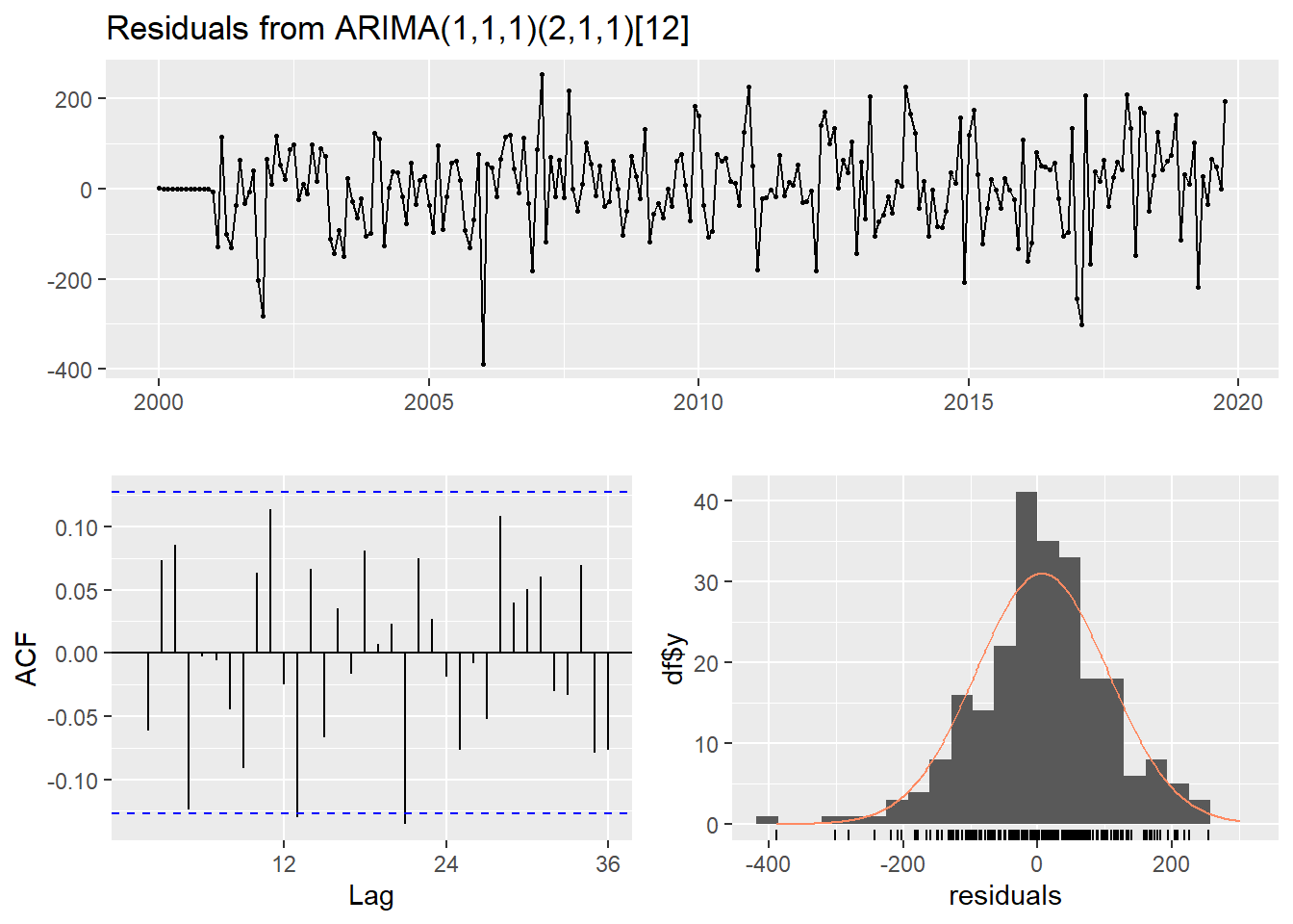


    Ljung-Box test

data:  Residuals from ARIMA(1,1,1)(2,1,1)[12]
Q* = 30.173, df = 19, p-value = 0.04964

Model df: 5.   Total lags used: 24

The output of the Ljung-Box test suggested that the residuals of the model are white noise.

By looking at the preceding residuals plot, you can see that the residuals are white noise and normally distributed. Furthermore, the Ljung-Box test confirms that there is no autocorrelation left on the residuals —with a p-value of 0.04, we cannot reject the null hypothesis that the residuals are white noise. We are good to go! Let’s use the forecast function to forecast the next 12 months of the USgas series:

USgas_fc <- forecast(final_md, h = 12)
# Plot the forecast
plot_forecast(USgas_fc,
              title = "US Natural Gas Consumption - Forecast",
              Ytitle = "Billion Cubic Feet",
              Xtitle = "Year")

41.7 The `auto.arima` function

One of the main challenges of forecasting with the ARIMA family of models is the cumbersome tuning process of the models. As we saw in this chapter, this process includes many manual steps that are required for verifying the structure of the series (stationary or non-stationary), data transformations, descriptive analysis with the $ACF$ and $PACF$ plots to identify the type of process, and eventually tune the model parameters. While it might take a few minutes to train an ARIMA model for a single series, it may not scale up if you have dozens of series to forecast.

The auto.arima function from the forecast package provides a solution to this issue. This algorithm automates the tuning process of the ARIMA model with the use of statistical methods to identify both the structure of the series (stationary or not) and type (seasonal or not), and sets the model’s parameters accordingly.

Example:

USgas_auto_md1 <- auto.arima(train)

Using the default arguments of the auto.arima function returns the $ARIMA$ model that minimizes the AIC score. In this case, a model was selected with an AIC score of $2599,67$:

USgas_auto_md1

Series: train 
ARIMA(2,1,1)(2,1,1)[12] 

Coefficients:
         ar1      ar2      ma1    sar1     sar2     sma1
      0.4301  -0.0372  -0.9098  0.0117  -0.2673  -0.7431
s.e.  0.0794   0.0741   0.0452  0.0887   0.0830   0.0751

sigma^2 = 10446:  log likelihood = -1292.83
AIC=2599.67   AICc=2600.22   BIC=2623.2

By default, the auto.arima function applies a shorter model search by using a step-wise approach for reducing the search time. The trade-off of this approach is that the model may miss some models that may achieve better results.

We can improvise with the auto.arima results by setting the search argument of the model. The stepwise argument, when set to FALSE, allows you to set a more robust and thorough search, with the cost of higher search time. This trade-off between performance and compute time can be balanced whenever you have prior knowledge about the series’ structure and characteristics.

Example:

# Retrain the training set of the USgas series again
USgas_auto_md2 <- auto.arima(train,
                             max.order = 5,
                             D = 1,
                             d = 1,
                             stepwise = FALSE,
                             approximation = FALSE)

You can see from the following results that with the robust search, the auto.arima algorithm returns the same model that was identified with the grid search we used in the Seasonal ARIMA model section:

USgas_auto_md2

Series: train 
ARIMA(1,1,1)(2,1,1)[12] 

Coefficients:
         ar1      ma1    sar1     sar2     sma1
      0.4247  -0.9180  0.0132  -0.2639  -0.7449
s.e.  0.0770   0.0376  0.0894   0.0834   0.0753

sigma^2 = 10405:  log likelihood = -1292.96
AIC=2597.91   AICc=2598.32   BIC=2618.08

41.8 Linear Regression with ARIMA Errors

One of the main assumptions of the linear regression model is that the error term of the series,$\epsilon$, is the white noise series (for example, there is no correlation between the residuals and their lags). However, when working with time series data, this assumption is violated as, typically, the model predictors do not explain all the variations of the series, and some patterns are left on the model residuals.

An example of the failure of this assumption can be seen while fitting a linear regression model to forecast the AirPassenger series. To illustrate this point, we will utilize the tslm function to regress the AirPassenger series with its trend, seasonal component, and seasonal lag (lag 12), and then evaluate the model residuals with the checkresiduals function.

Example:

df <- ts_to_prophet(AirPassengers)
names(df) <- c("date", "y")
df$lag12 <- dplyr::lag(df$y, n = 12)
library(lubridate)
df$month <- factor(month(df$date, label = TRUE), ordered = FALSE)
df$trend <- 1:nrow(df)

Now, we will split the series into training and testing partitions, leaving the last 12 months for testing using the ts_split function:

par <- ts_split(ts.obj = AirPassengers, sample.out = 12)
train <- par$train
test <- par$test

For the regression of the time series object with an external data.frame object (df), we will apply the same split for training and testing partitions on the predictor’s data.frame object:

train_df <- df[1:(nrow(df) - 12), ]
test_df <- df[(nrow(df) - 12 + 1):nrow(df), ]
# Train the model with the tslm function
md1 <- tslm(train ~ season + trend + lag12, data = train_df)

Let’s use the checkresiduals function to review the model’s residuals:

checkresiduals(md1)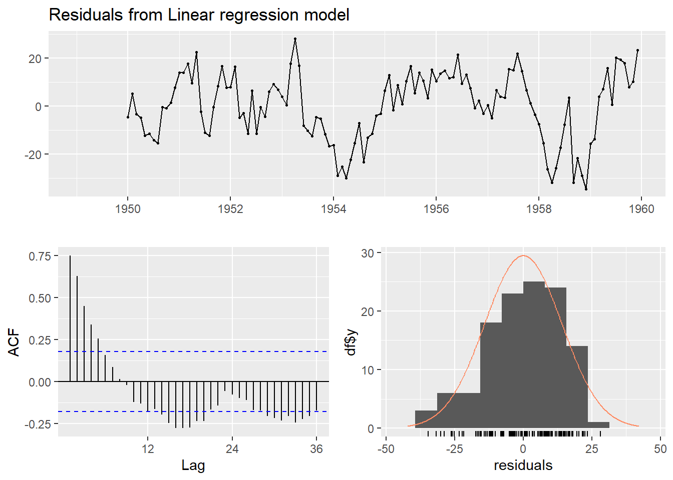


    Breusch-Godfrey test for serial correlation of order up to 24

data:  Residuals from Linear regression model
LM test = 83.147, df = 24, p-value = 1.903e-08

In the preceding ACF plot, the residuals series has a strong correlation with its past lags, and therefore the series is not white noise. We can conclude from the residuals plot that the regression model could not capture all the series patterns. Generally, this should not come as a surprise since the variation of the series could be affected by other variables, such as the ticket and oil prices, the unemployment rate, and other external factors.

A simple solution to this problem is to model the error terms with the $ARIMA$ model and add it to the regression.

41.8.1 Modeling the residuals with the ARIMA model

As we saw in the preceding ACF plot, the AirPassengers residuals indicate that the model was unable to capture all the patterns of the series. Another way to think about this is that the modeling of the series is not complete yet, and additional modeling can be applied on the model residuals to reveal the true error term of the model.

Let’s remodel the AirPassengers series, but this time with a linear regression model with ARIMA errors. While modeling the model’s error term with an ARIMA model, we should treat the residuals as a series by itself and set the model components $p$, $d$, and $q$ (and $P$, $D$, and $Q$ if the residuals series has seasonal component) using any of the approaches we introduced in this chapter (for example, manual tuning, grid search, or automating the search process with theauto.arima process). For simplicity, we will utilize the auto.arima function. The auto.arima function can be used to model a linear regression model with ARIMA errors via the use of the xreg argument:

Example:

md2 <- auto.arima(train,
                  xreg = cbind(model.matrix(~ month,train_df)[,-1],
                               train_df$trend,
                               train_df$lag12),
                  seasonal = TRUE,
                  stepwise = FALSE,
                  approximation = FALSE)

Note that the auto.arima and arima functions do not support categorical variables (that is, the factor class) with the xreg argument. Capturing the seasonal effect will require one-hot encoding (transforming each category into multiple binary variables) of the categorical variable.

Therefore, we used the model.matrix function from the stats package on the xreg argument of the auto.arima function to transfer the month variable from a categorical variable into a binary variable. In addition, we dropped the first column, which represents the first category (in this case, the month of January), to avoid the dummy variable trap.

We set the seasonal argument to TRUE to include a search of both non-seasonal and seasonal models. The auto.arima function will conduct a full search when the step-wise and approximation arguments are set to FALSE. Let’s use the summary function to review the model summary:

summary(md2)

Series: train 
Regression with ARIMA(2,0,0)(2,0,0)[12] errors 

Coefficients:
         ar1     ar2     sar1     sar2  monthfeb  monthmar  monthabr  monthmay
      0.5849  0.3056  -0.4421  -0.2063   -2.7523    0.8231    0.2066    2.8279
s.e.  0.0897  0.0903   0.1050   0.1060    1.8417    2.3248    2.4162    2.5560
      monthjun  monthjul  monthago  monthsep  monthoct  monthnov  monthdic
        6.6057   11.2337   12.1909    3.8269    0.6350   -2.2723   -0.9918
s.e.    3.2916    4.2324    4.1198    2.9243    2.3405    2.4211    1.9172
                    
      0.2726  1.0244
s.e.  0.1367  0.0426

sigma^2 = 72.82:  log likelihood = -426.93
AIC=889.86   AICc=896.63   BIC=940.04

Training set error measures:
                    ME     RMSE      MAE       MPE     MAPE      MASE
Training set 0.4117148 8.353629 6.397538 0.2571543 2.549682 0.2100998
                    ACF1
Training set 0.005966713

The auto.arima function regresses the series with the trend, month, and lag12 variables. In addition, the model used the AR(2) and SAR(2) processes for modeling the error term. We can now review the residuals of the modified md2 model with the checkresiduals functions:

checkresiduals(md2)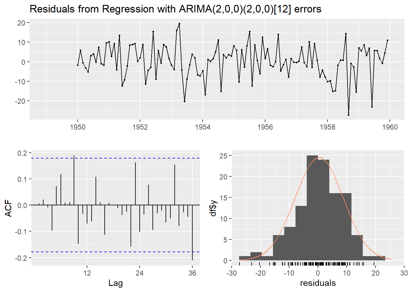


    Ljung-Box test

data:  Residuals from Regression with ARIMA(2,0,0)(2,0,0)[12] errors
Q* = 25.816, df = 20, p-value = 0.172

Model df: 4.   Total lags used: 24

You can see the change in the ACF plot after applying the linear regression model with ARIMA errors as the majority of the lags are not statistically significant, as opposed to the preceding linear regression model (md1).

Let’s evaluate the performance of both models (md1 and md2) on the testing set:

fc1 <- forecast(md1, newdata = test_df)
fc2 <- forecast(md2, xreg = cbind(model.matrix(~ month,test_df)[,-1],
                                  test_df$trend,
                                  test_df$lag12))

Now, let’s use the accuracy function to review the two model’s performance on both the testing and training partitions:

accuracy(fc1, test)

                        ME     RMSE      MAE        MPE     MAPE      MASE
Training set -1.894492e-15 13.99206 11.47136 -0.1200023 4.472154 0.3541758
Test set      1.079611e+01 20.82782 18.57391  1.9530865 3.828115 0.5734654
                  ACF1 Theil's U
Training set 0.7502578        NA
Test set     0.1653119 0.4052175

accuracy(fc2, test)

                      ME      RMSE       MAE        MPE     MAPE      MASE
Training set   0.4117148  8.353629  6.397538  0.2571543 2.549682 0.2100998
Test set     -11.2123706 17.928195 13.353910 -2.4898843 2.924174 0.4385521
                     ACF1 Theil's U
Training set  0.005966713        NA
Test set     -0.325044929 0.3923795

You can see from the output of the accuracy function that the linear regression with the $ARIMA$ model provides a significant improvement in the model’s accuracy with a lift of 43% on the $MAP$E score on the training set (from 4.5% to 2.5%) and 31% on the testing set (from 3.8% to 2.9%).

41.1 The Stationary Process

41.1.1 Stationary series

41.1.2 Non-stationary series

41.1.3 Transforming a non-stationary series into a stationary series

41.1.4 The random walk process

41.2 The AR Process

41.2.1 Example of AR process

41.2.2 Identifying the AR process and its characteristics

41.3 The MA Process

41.3.1 Example of MA process

41.3.2 Identifying the MA process and its characteristics

41.4 The ARMA model

41.4.1 Example of ARMA process

41.4.2 Identifying an ARMA process

41.5 The ARIMA model

41.5.1 Identifying an ARIMA process

41.5.2 Example of ARIMA process

41.6 The Seasonal ARIMA Model (SARIMA)

41.6.1 Forecasting US monthly natural gas consumption with the SARIMA model

41.7 The auto.arima function

41.8 Linear Regression with ARIMA Errors

41.8.1 Modeling the residuals with the ARIMA model

41.7 The `auto.arima` function