Forecasting is the third and last component of the time series analysis. Traditional time series forecasting follows the same workflow as most of the fields of predictive analysis, such as regression or classification, and typically includes the following steps:
Goal Definition. Determining and clearly defining the forecasting goal is essential for arriving at useful results. One must first determine the purpose of generating forecasts, the type of forecasts that are needed, how the forecasts will be used by the organization, what are the costs associated with forecast errors, what data will be available in the future, and more. These issues affect every step in the forecasting process, from data collection through data exploration, preprocessing, modeling and performance evaluation.
Descriptive vs. Predictive Goals. Time series data is done for either descriptive or predictive purposes. In descriptive modeling, or time series analysis, a time series is modeled to determine its components in terms of seasonal patterns, trends, relation to external factors, and the like. These can then be used for decision making and policy formulation. In contrast, time series forecasting uses the information in a time series (perhaps with additional information) to forecast future values of that series. The difference between descriptive and predictive goals leads to differences in the types of methods used and in the modeling process itself. A predictive model is judged by its predictive accuracy rather than by its ability to provide correct causal explanations.
Forecast Horizon and Forecast Updating. How far into the future should we forecast? Must we generate all forecasts at a single time point, or can forecasts be generated on an ongoing basis?. Both questions depend on how the forecasts will be used in practice and therefore require close collaboration with the forecast stakeholders in the organization. While long-term forecasting is often a necessity, it is important to have realistic expectations regarding forecast accuracy: the further into the future, the more likely that the forecasting context will change and therefore uncertainty increases. The model should be examined periodically to assure its suitability for the changed context and if possible, updated. Therefore, it is sometimes useful to provide periodic updated forecasts by incorporating new accumulated information. Such refreshing of the forecasts based on new data is called roll-forward forecasting. All these aspects of the forecast horizon have implications on the required length of the series for building the forecast model, on frequency and timeliness of collection, on the forecasting methods used, on performance evaluation, and on the uncertainty levels of the forecasts.
Forecast Use. How will the forecasts be used? Understanding how the forecasts will be used, perhaps by different stakeholders, is critical for generating forecasts of the right type and with a useful accuracy level. Will the forecasts and forecasting method to be presented to management or to the technical department? Answers to such questions are necessary for choosing appropriate data, methods, and evaluation schemes.
Level of Automation. The level of required automation depends on the nature of the forecasting task and on how forecasts will be used in practice. In scenarios where many series are to be forecasted on an ongoing basis, and not much forecasting expertise can be allocated to the process, an automated solution can be advantageous.
Data preparation: Here, we prepare the data for the training and testing process of the model. This step includes splitting the series into training (in-sample) and testing (out-sample) partitions, creating new features (when applicable), and applying a transformation if needed (for example, log transformation, scaling, and so on).
Data Quality. The quality of our data in terms of measurement accuracy, missing values, corrupted data, and data entry errors can greatly affect the forecasting results. Data quality is especially important in time series forecasting, where the sample size is small (typically not more than a few hundred values in a series).
Temporal Frequency. With today’s technology, many time series are recorded on very frequent time scales. However, although data might be available at a very frequent scale, for the purpose of forecasting it is not always preferable to use this frequency. In considering the choice of temporal frequency, one must consider the frequency of the required forecasts (the goal) and the level of noise1 in the data. For example, if the goal is to forecast next-day sales at a grocery store, minute-by-minute sales data is likely less useful than daily aggregates, and the minute-by-minute series will contain many sources of noise that degrade its daily-level forecasting power. Even when forecasts are needed on a particular frequency (such as daily) it is sometimes advantageous to aggregate the series to a lower frequency (such as weekly), and model the aggregated series to produce forecasts.
Series Granularity. “Granularity” refers to the coverage of the data. This can be in terms of geographical area, population, time of operation, etc. As with temporal frequency, the level of granularity must be aligned with the forecasting goal, while considering the levels of noise. Exploring different aggregation and slicing levels is often needed for obtaining adequate series. The level of granularity will eventually affect the choice of preprocessing, forecasting method(s), and evaluation metrics.
Domain Expertise. Domain expertise is needed for determining which data to use (e.g., daily vs. hourly, how far back, and from which source), describing and interpreting patterns that appear in the data, from seasonal patterns to extreme values and drastic changes (e.g., clarifying what are “after hours”, interpreting massive absences due to the organization’s annual picnic, and explaining the drastic change in trend due to a new company policy). Domain expertise is also used for helping evaluate the practical implications of the forecasting performance.
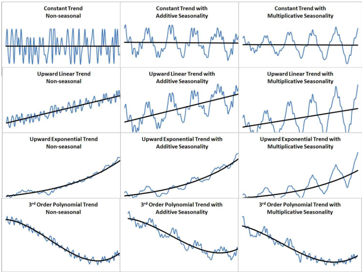
Time Series Components. For the purpose of choosing adequate forecasting methods, it is useful to dissect a time series into a systematic part and a non-systematic part. The systematic part is typically divided into three components: level, trend, and seasonality. The non-systematic part is called noise.
Level describes the average value of the series, trend is the change in the series from one period to the next, and seasonality describes a short-term cyclical behavior that can be observed several times within the given series. While some series do not contain trend or seasonality, all series have a level. Lastly, noise is the random variation that results from measurement error or other causes that are not accounted for. It is always present in a time series to some degree, although we cannot observe it directly.
The different components are commonly considered to be either additive or multiplicative. Forecasting methods attempt to isolate the systematic part and quantify the noise level. The systematic part is used for generating point forecasts and the level of noise helps assess the uncertainty associated with the point forecasts.
Visualizing Time Series. An effective initial step for characterizing the nature of a time series and for detecting potential problems is to use data visualization. By visualizing the series we can detect initial patterns, identify its components and spot potential problems such as extreme values, unequal spacing, and missing values.
Missing Values. Missing values in a time series create “holes” in the series. The presence of missing values has different implications and requires different actions depending on the forecasting method. Forecasting methods such as ARIMA models and smoothing methods cannot be directly applied to time series with missing values, because the relationship between consecutive periods is modeled directly. In such cases, a solution is to impute, or “fill in”, the missing values. Imputation approaches range from simple solutions, such as averaging neighboring values, to creating forecasts of missing values using earlier values or external data. In contrast, forecasting methods such as linear and logistic regression models and neural networks can be fit to a series with “holes”, and no imputation is required. The implication of missing values in such cases is that the model/method is fitted to less data points. In short, since some forecasting methods cannot tolerate missing values in a series and others can, it is important to discover any missing values before the modeling stage.
Unequally Spaced Series. Equal spacing means that the time interval between two consecutive periods is equal (e.g., daily, monthly, quarterly data). However, some series are naturally unequally spaced. These include series that measure some quantity during events where event occurrences are random (such as bus arrival times), naturally unequally spaced (such as holidays or music concerts), or determined by someone other than the data collector (e.g., bid timings in an online auction). As with missing values, some forecasting methods can be applied directly to unequally spaced series, while others cannot. Converting an unequally spaced series into an equally spaced series typically involves interpolation using approaches similar to those for handling missing values.
Extreme values. These are values that are unusually large or small compared to other values in the series. Extreme values can affect different forecasting methods to various degrees. The decision whether to remove an extreme value or not must rely on information beyond the data. Is the extreme value the result of a data entry error? Was it due to an unusual event (such as an earthquake) that is unlikely to occur again in the forecast horizon? If there is no grounded justification to remove or replace the extreme value, then the best practice is to generate two sets of forecasts: those based on the series with the extreme values and those based on the series excluding the extreme values.
Choice of Time Span. Another pre-processing operation that is sometimes required is determining how far back into the past we should be consider. In other words, what is the time span of the data to be used. While a very short (and recent) series might be insufficiently informative for forecasting purposes, beyond a certain length the additional information will likely be useless at best, and harmful at worst. Considering a very long past of the series might deteriorate the accuracy of future forecasts because of the changing context and environment occurring during the data period.
Train the model: When building predictive models we typically create two or three data partitions: a training set, a validation set, and sometimes an additional test set. The training partition, typically the largest partition, contains the data used to train, tune, and estimate the model coefficients that minimize the selected error criteria. The same training partition is generally used to develop multiple models. The fitted values and the model estimation of the training partition observations will be used later on to evaluate the overall performance of the model. The validation partition is used to assess the performance of each model so that we can compare models and pick the best one. The test partition (sometimes called the hold- out or evaluation partition) is used to assess the performance of the chosen model with new data. Before attempting to forecast future values of the series, the training and validation periods must be recombined into one long series, and the chosen method/model is rerun on the complete data. This final model is then used to forecast future values.
Test the model: Here, we utilize the trained model to forecast the corresponding observations of the testing partition. The main idea here is to evaluate the performance of the model with a new dataset (that the model did not see during the training process).
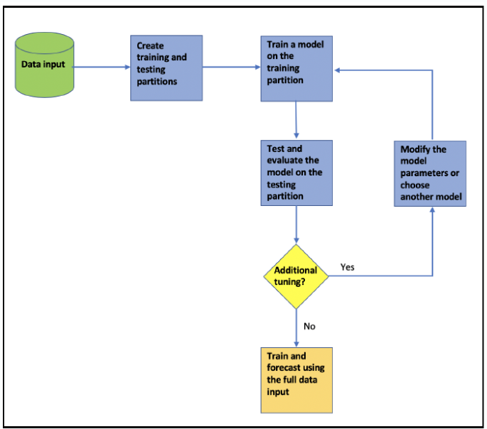
Model evaluation: Last but not least, after the model was trained and tested, it is time to evaluate the overall performance of the model on both the training and testing partitions. Based on the evaluation process of the model, if the model meets a certain threshold or criteria, then we either retain the model using the full series in order to generate the final forecast or select a new training parameter/different model and repeat the training process.
Note that the process does not end once forecasts are generated, because forecasting is typically an ongoing goal. Hence, forecast accuracy is monitored and sometimes the forecasting method is adapted or changed to accommodate changes in the goal or the data over time.
In time series, this process has its own unique characteristics, which distinguish it from other predictive fields:
The training and testing partitions must be ordered in chronological order, as opposed to random sampling.
Once we have trained and tested the model using the training and testing partitions, we will retrain the model with all of the data (or at least the most recent observation in chronological order).
Figure 14. Time series forecasting workflow
37.2 Training Approaches
One of the core elements of the forecasting workflow is the model training process. The quality of the model’s training will have a direct impact on the forecast output. The main goals of this process are as follows:
Formalize the relationship of the series with other factors, such as seasonal and trend patterns, correlation with past lags, and external variables in a predictive manner.
Tune the model parameters (when applicable).
Check if the model is scalable on new data, or in other words, avoids overfitting.
Prior to the training process, the series is split into training and testing partitions, where the model is being trained on the training partition and tested on the testing partition. These partitions must be in chronological order, regardless of the training approach that has been used. The main reason for this is that most of the time series models establish a mathematical relationship between the series in terms of its past lags and error terms.
37.2.1 Training with single training and testing partitions
One of the most common training approaches is using single training and testing (or single out-of-sample) partitions. This approach is based on splitting the series into training and testing partitions (or in-sample and out-sample partitions, respectively), training the model on the training partition, and testing its performance on the testing set.
This approach has a single parameter —the length of the out-of-sample (or the length of the testing partition). Typically, the length of the testing partition is derived from the following rules of thumb: up to 30% of the total length of the series in order to have enough observation data for the training process.
There are two methods to split a time series into a training and testing partitions:
The window method.
Example:
Split the USgas series into partitions, leaving the last 12 observations of the series as the testing partition and the rest as training.
library(TSstudio)data(USgas)ts_info(USgas)
 The USgas series is a ts object with 1 variable and 238 observations
 Frequency: 12
 Start time: 2000 1
 End time: 2019 10
# Use the window function to split the series into training and testing# partitionstrain <-window(USgas, start =time(USgas)[1], end =time(USgas)[length(USgas) -12])test <-window(USgas,start =time(USgas)[length(USgas) -12+1],end =time(USgas)[length(USgas)])ts_info(train)
 The train series is a ts object with 1 variable and 226 observations
 Frequency: 12
 Start time: 2000 1
 End time: 2018 10
ts_info(test)
 The test series is a ts object with 1 variable and 12 observations
 Frequency: 12
 Start time: 2018 11
 End time: 2019 10
The ts_split function from the TSstudio package, which provides a customized way for creating training and testing partitions for time series data:
 The train series is a ts object with 1 variable and 226 observations
 Frequency: 12
 Start time: 2000 1
 End time: 2018 10
ts_info(test)
 The test series is a ts object with 1 variable and 12 observations
 Frequency: 12
 Start time: 2018 11
 End time: 2019 10
The main advantage of this method is its simplicity, as it is fairly fast to train and test a model while using (relatively) cheap compute power. On the other hand, it isn’t possible to come to a conclusion about the stability and scalability of the model’s performance based on a single test unit. One way to mitigate that risk is with the backtesting approach, which is based on training a model with multiple training and testing partitions.
37.2.2 Training with backtesting
The backtesting approach for training a forecasting model is an advanced version of the single out-of-sample approach we saw previously. It is based on the use of a rolling window to split the series into multiple pairs of training and testing partitions.
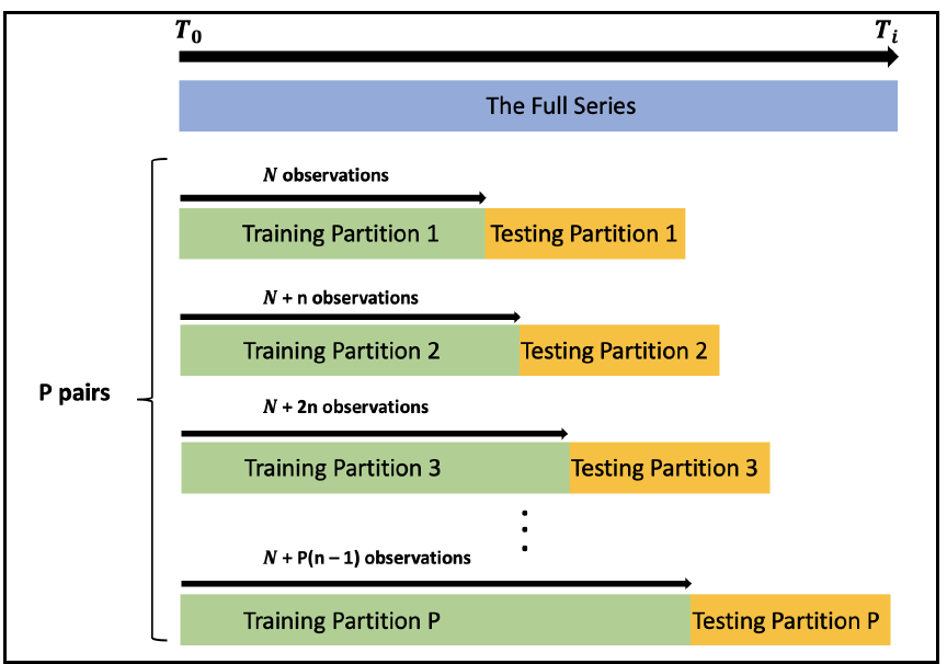
The following diagram demonstrates the structure of the backtesting with an expanding window:
Figure 15. The backtesting training process
As you can see in the preceding diagram, all of the training partitions of the expanding window method start at the same index point, \(T_0\), where each training partition is a combination of the previous training partition with the following \(n\) observations (where \(n\) is a constant that represents the expanded rate of the window). It would make sense to use this method when the series has a strong seasonal pattern and stable trend. In this case, the first observations of the series could, potentially, have predictive information that can be utilized by the model.
The downside of this method is training the model with different length partitions, as typically a model tends to learn more and therefore perform better when more data is available. Therefore, we may observe that the performance of models that are trained on the latest partitions perform better than the ones that are trained with the first partitions.
37.3 Forecast Methods
There is a big variety of forecasting methods for time series, the reason being is that different methods perform differently depending on the nature of the data and the forecasting requirements. Forecasting methods can be roughly divided into the following:
Model-based methods. This methods use a statistical, mathematical, or other scientific model to approximate a data series. The training data are used to estimate the parameters of the model, and then the model with estimated parameters is used to generate forecasts. Model-based forecasting methods include multiple linear regression and autoregressive models, where the user specifies a certain linear model and then estimates it from the time series. Logistic regression models are also model-based. Model-based methods are especially advantageous when the series at hand is very short.
Data-driven methods. These methods include data-driven approach of smoothing, where algorithms “learn” patterns from the data. Data-driven methods are advantageous when model assumptions are likely to be violated, or when the structure of the time series changes over time. Naive forecasts are also data-driven, in that they simply use the last data point in the series for generating a forecast. Another advantage of many data-driven forecasting methods is that they require less user input, however, this means that more data (that is, a longer series) is required for adequate learning. Data mining methods such as neural networks, regression trees and other algorithms for predicting cross-sectional data are sometimes used for time series forecasting, especially for incorporating external information into the forecasts.
Model-based methods are generally preferable for forecasting series with global patterns that extend throughout the data period, as they use all the data to estimate the global pattern. For a local pattern, a model would require specifying how and when the patterns change, which is usually impractical and often unknown. Therefore, data-driven methods are preferable for forecasting series with local patterns, as they “learn” patterns from the data, and their memory length can be set to best adapt to the rate of change in the series.
Note that one serious danger with data-driven methods is overfitting the training period, and hence performance should be carefully evaluated and constantly monitored to avoid this pitfall.
The methods presented here create forecasts for a time series based on its history. Such methods are termed extrapolation methods. The advantage of this practice is simplicity. The disadvantage is that forecasts do not take into account possible relationships between the series. An alternative to extrapolation methods, when the purpose is forecasting, is to capture external information that correlates with a series more heuristically. For example, consider a model for forecasting the average weekly airfare on a certain route that adds to the model the weekly gas prices and past weekly airfare rates as inputs.
37.3.1 Forecasting automation
In terms of automation, some forecasting methods are easier to automate than others. Typically, data-driven methods are easier to automate, because they “learn” patterns from the data. However, even data-driven methods can perform poorly if the characteristics of the series (seasonality, trend) are not correctly specified, or if there is insufficient data.
Smoothing methods are preferable for automated forecasting, because they require less tweaking, are suitable for a range of trends and seasonal patterns, are computationally fast, require very little data storage, and adjust when the behavior of a series changes over time.
Neural networks are similarly useful for automation, although they are computationally more demanding and require a lot of past data.
Even with an automated system in place, it is advisable to monitor the forecasts and forecast errors produced by an automated system and occasionally re-examine their suitability and update the system accordingly.
37.3.2 Combining methods
While it might appear that we should choose one method for forecasting among the various options, it turns out that combining multiple forecasting methods can lead to improved predictive performance.
Combining methods can be done via two-level (or multilevel) methods, where the first method uses the original time series to generate forecasts of future values, and the second method uses the forecast errors from the first layer to generate forecasts of future forecast errors, thereby “correcting” the first level forecasts.
Another combination approach is via ensembles, where multiple methods are applied to the time series, each generating separate forecasts. The resulting forecasts are then averaged in some way to produce the final forecast. Averaging across multiple methods can lead to forecasts that are more robust and are of higher precision.
Another combination approach is to use different series measuring the same phenomenon of interest (e.g., temperature) and take an average of the multiple resulting forecasts. For example, when a series of interest is available from multiple sources, each with slightly different numbers or precision (e.g., from manual and electronic collection systems or from different departments or measuring devices), we can create ensembles of forecasts, each based on a different series.
37.4 Forecast Evaluation
The primary goal of the evaluation step is to assess the ability of the trained model to forecast (or based on other criteria) the future observations of the series accurately. This process includes doing the following:
Residual analysis: This focuses on the quality of the model, with fitted values in the training partition.
Scoring the forecast: This is based on the ability of the model to forecast the actual values of the testing set.
37.4.1 Residual analysis
Residual analysis tests how well the model captured and identified the series patterns. In addition, it provides information about the residuals distributions, which are required to build confidence intervals for the forecast.
The mathematical definition of a residual is the difference between the actual observation and the corresponding fitted value of the model, which was observed in the training process, or as the following equation:
\[\epsilon_t = Y_t - \hat{Y_t}\]
Where, \(\epsilon_t\), \(Y_t\), and \(\hat{Y_t}\) represent the residual, actual, and fitted values, respectively, at time \(t\).
To demonstrate the residual analysis process, we will train an ARIMA model on the training partition we created earlier for the USgas series.
Example:
library(forecast)md <-auto.arima(train)
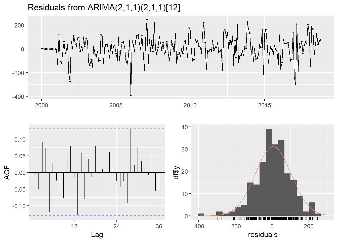
The checkresiduals function from the forecast package returns the following four outputs:
Time series plot of the residuals.
ACF plot of the residuals.
Distribution plot of the residuals.
The output of the Ljung-Box test. Recall that the Ljung-Box test is a statistical method for testing whether the autocorrelation of a series (which, in this case, is the residuals) is different from zero.
checkresiduals(md)
    Ljung-Box test

data:  Residuals from ARIMA(2,1,1)(2,1,1)[12]
Q* = 24.95, df = 18, p-value = 0.1263

Model df: 6.   Total lags used: 24
Starting with the output of the Ljung-Box test output, you will notice that, based on the P-value results, we can reject the null hypothesis with a level of significance of 0.01. Hence, there is an indication that the correlation between the residual series and its lags are different from zero.
The ACP plot provides additional support for that as well. This indicates that the model did not fully capture all of the series patterns, and you may want to modify the model tuning parameters.
The residual time series plot oscillates around the x-axis, with the exception of a few residuals, which cross the value of +/- 200. This could indicate that some outliers occur during these periods, and you should check those data points in the series.
Last but not least is the distribution plot of the residuals, which seem to be a fairly good representation of a normal distribution.
37.4.2 Scoring the forecast
Once you finalize the model tuning, it is time to test the ability of the model to predict observations that the model didn’t see before (as opposed to the fitted values that the model saw throughout the training process). The most common method for evaluating the forecast’s success is to predict the actual values with the use of an error metric to quantify the forecast’s overall accuracy.
The selection of a specific error metric depends on the forecast accuracy’s goals. Common examples of common error metrics are: the Mean Squared Error (MSE), the Root Mean Squared Error (RMSE), the Mean Absolute Error (MAE), the Mean Absolute Percentage Error (MAPE).
We will use the accuracy function to obtain several error metrics for both the fitted values (the training set row) and the actual forecast (the test set row).
Example:
Use the model we trained earlier (md) to forecast the 12 observations we left for testing and score its performance.
fc <-forecast(md, h =12)# Score the model's performance with respect to the actual values# in the testing partition:accuracy(fc, test)
                    ME      RMSE      MAE       MPE     MAPE      MASE
Training set  5.844136  97.81626 73.42657 0.1170672 3.522348 0.6376860
Test set     37.847885 103.22848 81.46603 1.3107987 3.261643 0.7075062
                     ACF1 Theil's U
Training set -0.004183172        NA
Test set     -0.046708926 0.3404092
You will notice that the model MAPE results are 3.52% and 7.84% on the training and testing partitions, respectively. A higher error rate on the testing partition compared to the training partition should not come as a surprise, as typically the model saw the training partition data throughout the training process. A fairly low error rate in the training set, along with the high error rate in the testing set, is a clear indication of overfitting in the model.
An alternative approach to evaluating the fit of the model on both the training and testing is with the test_forecast function from the TSstudio package. This function visualizes the actual series, the fitted values on the training partition, and the forecasted values on the testing set. Hovering over the fitted or forecasted values makes a textbox pop up with the RMSE and MAPE results on both the training and testing partitions.
With this approach it is easier and faster to identify insights about the goodness of the fit of both the fitted and forecasted values when plotting those values against the actual values of the series. For instance, you will immediately notice that the residual peak during 2006 is caused by outliers (or lower consumption than the normal pattern of the series). In addition, the actual forecast missed the 2018 yearly peak. Those insights cannot be observed with error metrics.
37.4.3 Forecast benchmark
According to the error metrics, the trained model scored a MAPE of 3.26% or RMSE of 103.221. How can we assess whether these results are too high or low? The most common method is to benchmark the model’s performance to some baseline forecast or to some legacy method that we wish to replace.
A popular benchmark approach would be to use a simplistic forecasting approach as a baseline. For instance, let’s forecast the series with a naive approach and use it as a benchmark for the previous forecast we created with the ARIMA model.
Example:
library(forecast)naive_model <-naive(train, h =12)
A naive approach typically assumes that the most recently observed value is the true representative of the future. Therefore, it will continue with the last value to infinity (or as the horizon of the forecast). In the naive model, there is no training process, and the fitted values are set as the actual values.
# Review the performance of the model on the training and testing partitionstest_forecast(actual = USgas,forecast.obj = naive_model,test = test)
# Evaluate the model's performance on both the training and testing partitionsaccuracy(naive_model, test)
                     ME     RMSE      MAE        MPE     MAPE     MASE
Training set  -1.028444 285.6607 228.5084 -0.9218463 10.97123 1.984522
Test set     301.891667 499.6914 379.1417  9.6798015 13.28187 3.292723
                  ACF1 Theil's U
Training set 0.3761105        NA
Test set     0.7002486  1.499679
However, since USgas has a strong seasonal pattern, it would make sense to use a seasonal naive model that takes into account seasonal variation. The snaive_model function from the forecast package uses the last seasonal point as a forecast of all of the corresponding seasonal observations. For example, if we are using monthly series, the value of the most recent January in the series will be used as the point forecast for all future January months:
snaive_model <-snaive(train, h =12)test_forecast(actual = USgas,forecast.obj = snaive_model,test = test)
# Evaluate the model's performance on both the training and testing partitionsaccuracy(snaive_model, test)
                   ME     RMSE      MAE      MPE     MAPE     MASE       ACF1
Training set 33.99953 148.7049 115.1453 1.379869 5.494048 1.000000  0.4859501
Test set     96.45000 164.6967 135.8833 3.612060 5.220458 1.180103 -0.2120929
             Theil's U
Training set        NA
Test set     0.4289964
It seems that the seasonal naive model has a better fit for the type of series we are forecasting, that is, USgas, due to its strong seasonal pattern (compared to the naive model). Therefore, we will use it as a benchmark for the ARIMA model.
By comparing both the MAPE and RMSE of the two models in the testing partition, it is clear that the ARIMA model provides a lift (in terms of accuracy) with respect to the benchmark model:
Model
MAPE
RMSE
ARIMA
3.26%
103.22
snaive
5.22%
164.69
37.5 Finalizing the Forecast
Now that the model has been trained, tested, tuned (if required), and evaluated successfully, we can move forward to the last step and finalize the forecast. This step is based on recalibrating the model’s weights or coefficients with the full series.
There are two approaches to using the model parameter setting:
If the model was tuned manually, you should use the exact tuning parameters that were used on the trained model.
If the model was tuned automatically by an algorithm (such as the auto.arima), you can do either of the following:
Extract the parameter setting that was used by with the training partition.
Let the algorithm retun the model parameters using the full series, under the assumption that the algorithm has the ability to adjust the model parameters correctly when training the model with new data. The use of algorithms to automate the model tuning process is recommended when the model’s ability to tune the model is tested with backtesting.
Example:
md_final <-auto.arima(USgas)fc_final <-forecast(md_final, h =12)plot_forecast(fc_final,title ="The US Natural Gas Consumption Forecast",Xtitle ="Year",Ytitle ="Billion Cubic Feet")
37.6 Handling Forecast Uncertainty
The main goal of the forecasting process is to minimize the level of uncertainty around the future values of the series. Although we cannot completely eliminate this uncertainty, we can quantify it and provide some range around the point estimate of the forecast (which is nothing but the model’s expected value of each point in the future). This can be done by using either the confidence interval (or a credible interval, when using the Bayesian model) or by using simulation.
37.6.1 Confidence intervals
The confidence interval is a statistical approximation method that’s used to express the range of possible values that contain the true value with some degree of confidence (or probability).
There are two parameters that determine the range of confidence interval:
The level of confidence or the probability that the true value will be in that range. The higher the level of confidence is, the wider the interval range. By default, the forecast function generates a prediction interval with a level of confidence of 80% and 95%, but you can modify it using the level argument.
The estimated standard deviation of the forecast at time \(T+i\), where \(T\) represents the length of the series and \(i\) represents the \(i\) forecasted value. The lower the error rate, the shorter the range of the prediction interval.
Example:
fc_final2 <-forecast(md_final, h =60, level =c(80, 90))plot_forecast(fc_final2,title ="The US Natural Gas Consumption Forecast",Xtitle ="Year",Ytitle ="Billion Cubic Feet")
37.6.2 Simulation
An alternative approach is to use the model distribution to simulate possible paths for the forecast. This method can only be used when the model distribution is available.
The forecast_sim function from the TSstudio package provides a built-in function for simulating possible forecasting paths. This estimate can be used to calculate the forecast point estimate (for example, using the mean or median of all of the paths), or to calculate probabilities of getting different values.
Example:
# Feed the same model to the function and run 500 iterations:fc_final3 <-forecast_sim(model = md_final,h =60,n =500)
fc_final3 contains all of the calculate simulations and the simulated paths. Let’s extract the simulation plot (and use the plotly package to add titles for the plot):
The horse race approach is a robust forecasting approach based on training, testing, and evaluating multiple forecasting models and selecting the model that performs the best on the testing partitions.
In the following example, we will apply horse racing between seven different models using backtesting. The train_model function from the TSstudio package conducts the full process of training, testing, evaluating, and then forecasting, using the model that performed the best on the backtesting testing partitions. By default, the model will test the following models:
arima - model from the stats package
auto.arima - Automated ARIMA model. from the forecast package
ets - Exponential smoothing state space model from the forecast package
HoltWinters - Holt-Winters filtering from the stats package
nnetar - Neural network time series model from the forecast package
tslm - model from the forecast package (note that the ‘tslm’ model must have the formula argument in the ‘method_arg’ argument)
Example:
library(TSstudio)set.seed(1234)methods <-list(ets1 =list(method ="ets",method_arg =list(opt.crit ="lik"),notes ="ETS model with opt.crit = lik"),ets2 =list(method ="ets",method_arg =list(opt.crit ="amse"),notes ="ETS model with opt.crit = amse"),arima1 =list(method ="arima",method_arg =list(order =c(2,1,0)),notes ="ARIMA(2,1,0)"),arima2 =list(method ="arima",method_arg =list(order =c(2,1,2),seasonal =list(order =c(1,1,1))), notes ="SARIMA(2,1,2)(1,1,1)"),hw =list(method ="HoltWinters",method_arg =NULL,notes ="HoltWinters Model"),tslm =list(method ="tslm",method_arg =list(formula = input ~ trend + season),notes ="tslm model with trend and seasonal components"))USgas_forecast <-train_model(USgas, methods = methods,train_method=list(partitions =4, sample.out =12, space =3),error ="MAPE",horizon =60)
The model provides a leaderboard that’s ordered based on the error criteria that’s set. In this case, the hw model had the lowest error rate, and therefore the function recommended that we use it (although all of the models and their forecasts are available for extraction from the function output).