20 Functions

Functions are one of the main building blocks for large programs: they are an essential tool for structuring complex algorithms. Arguably one of R’s strengths as a tool for scientific programming is the ease with which it can be extended for specific purposes, using functions written by the R community and made available as R packages.

The most important advantage of using a function is that once it is loaded, it can be used again and again without having to reload it. User-defined functions can be used in the same way as predefined functions are used in R. In particular they can be used within other functions.

The second most important use of functions is to break down a programming task into smaller logical units. Large programs are typically made up of a number of smaller functions, each of which does a simple well-defined task.

20.1 Building Functions

Functions are often used to encapsulate a sequence of expressions that need to be executed numerous times, perhaps under slightly different conditions. Functions are also often written when code must be shared with others or the public.

The writing of a function allows a developer to create an interface to the code, that is explicitly specified with a set of parameters.

A function has the general form:

name <- function(argument_1, argument_2, ...) {
  expression_1
  expression_2
  <some other expressions>
  return(output)
}

Here argument_1, argument_2, etc., are the names of variables and expression_1, expression_2, and output are all regular R expressions.

name is the name of the function. Because all function arguments have names, they can be specified using their name. Specifying an argument by its name is sometimes useful if a function has many arguments and it may not always be clear which argument is being specified.

Example:

f(num = 2)

Some functions may have no arguments, and that the braces are only necessary if the function comprises more than one expression.

Example:

f <- function(num = 1) {   
## if the function is called without the num argument being explicitly specified, then it will print “Hello, world!” to the console once.
  hello <- "Hello, world!\n" 
  for(i in seq_len(num)) {
    cat(hello)
  }
  chars <- nchar(hello) * num 
  chars
}

In R, the return value of a function is always the very last expression that is evaluated (in the example is chars).

The formals() function returns a list of all the formal arguments of a function.

Note that functions have their own class.

20.1.1 Vector functions

Vector functions take one or more vectors and return a vector result. For example, take a look at this code. What does it do?

df <- tibble(
  a = rnorm(5),
  b = rnorm(5),
  c = rnorm(5),
  d = rnorm(5),
)

df |> mutate(
  a = (a - min(a, na.rm = TRUE)) / 
    (max(a, na.rm = TRUE) - min(a, na.rm = TRUE)),
  b = (b - min(b, na.rm = TRUE)) / 
    (max(b, na.rm = TRUE) - min(b, na.rm = TRUE)),
  c = (c - min(c, na.rm = TRUE)) / 
    (max(c, na.rm = TRUE) - min(c, na.rm = TRUE)),
  d = (d - min(d, na.rm = TRUE)) / 
    (max(d, na.rm = TRUE) - min(d, na.rm = TRUE)),
)

# A tibble: 5 × 4
      a     b     c     d
  <dbl> <dbl> <dbl> <dbl>
1 0.763 0.613 1     0.762
2 1     1     0.396 0    
3 0.461 0.467 0     0.347
4 0.431 0.226 0.632 1    
5 0     0     0.601 0.493

To write a function you need to first analyse your repeated code to figure what parts are constant and what parts vary. If we take the code above and pull it outside of mutate(), it’s a little easier to see the pattern because each repetition is now one line:

(█ - min(█, na.rm = TRUE)) / (max(█, na.rm = TRUE) - min(█, na.rm = TRUE))

Then you create a function by following the template:

name <- function(arguments) {
  body
}

Example:

rescale01 <- function(x) {
  (x - min(x, na.rm = TRUE)) / (max(x, na.rm = TRUE) - min(x, na.rm = TRUE))
}

You might test with a few simple inputs to make sure you’ve captured the logic correctly:

rescale01(c(-10, 0, 10))

[1] 0.0 0.5 1.0

Then you can rewrite the call to mutate() as:

df |> mutate(
  a = rescale01(a),
  b = rescale01(b),
  c = rescale01(c),
  d = rescale01(d),
)

# A tibble: 5 × 4
      a     b     c     d
  <dbl> <dbl> <dbl> <dbl>
1 0.763 0.613 1     0.762
2 1     1     0.396 0    
3 0.461 0.467 0     0.347
4 0.431 0.226 0.632 1    
5 0     0     0.601 0.493

20.1.2 Data frames functions

Data frame functions work like dplyr verbs: they take a data frame as the first argument, some extra arguments that say what to do with it, and return a data frame or a vector.

When you start writing functions that use dplyr verbs you rapidly hit the problem of indirection. Let’s illustrate the problem with a very simple function: grouped_mean(). The goal of this function is to compute the mean of mean_var grouped by group_var:

Example:

grouped_mean <- function(df, group_var, mean_var) {
  df |> 
    group_by(group_var) |> 
    summarize(mean(mean_var))
}

If we try and use it, we get an error:

diamonds |> grouped_mean(cut, carat)

#> Error in `group_by()`:
#> ! Must group by variables found in `.data`.
#> ✖ Column `group_var` is not found.

Here we need some way to tell group_by() and summarize() not to treat group_var and mean_var as the name of the variables, but instead look inside them for the variable we actually want to use.

So to make grouped_mean() work, we need to surround group_var and mean_var with { }. Embracing a variable tells dplyr to use the value stored inside the argument, not the argument as the literal variable name. One way to remember what’s happening is to think of { } as looking down a tunnel — { var } will make a dplyr function look inside of var rather than looking for a variable called var.

Example:

grouped_mean <- function(df, group_var, mean_var) {
  df |> 
    group_by({{ group_var }}) |> 
    summarize(mean({{ mean_var }}))
}

diamonds |> grouped_mean(cut, carat)

# A tibble: 5 × 2
  cut       `mean(carat)`
  <ord>             <dbl>
1 Fair              1.05 
2 Good              0.849
3 Very Good         0.806
4 Premium           0.892
5 Ideal             0.703

So the key challenge in writing data frame functions is figuring out which arguments need to be embraced. Fortunately, this is easy because you can look it up from the documentation.

20.1.3 Plot functions

You might want to return a plot. For example, imagine that you’re making a lot of histograms:

diamonds |> 
  ggplot(aes(x = carat)) +
  geom_histogram(binwidth = 0.1)

diamonds |> 
  ggplot(aes(x = carat)) +
  geom_histogram(binwidth = 0.05)

Wouldn’t it be nice if you could wrap this up into a histogram function? This is easy as pie once you know that aes() is a data-masking function and you need to embrace:

histogram <- function(df, var, binwidth = NULL) {
  df |> 
    ggplot(aes(x = {{ var }})) + 
    geom_histogram(binwidth = binwidth)
}

diamonds |> histogram(carat, 0.1)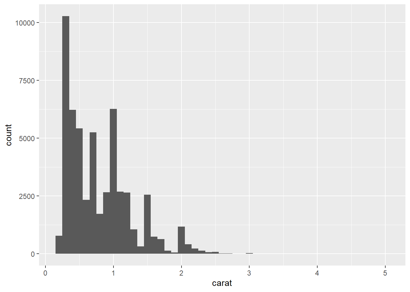

Note that histogram() returns a ggplot2 plot, meaning you can still add on additional components if you want. Just remember to switch from |> to +:

diamonds |> 
  histogram(carat, 0.1) +
  labs(x = "Size (in carats)", y = "Number of diamonds")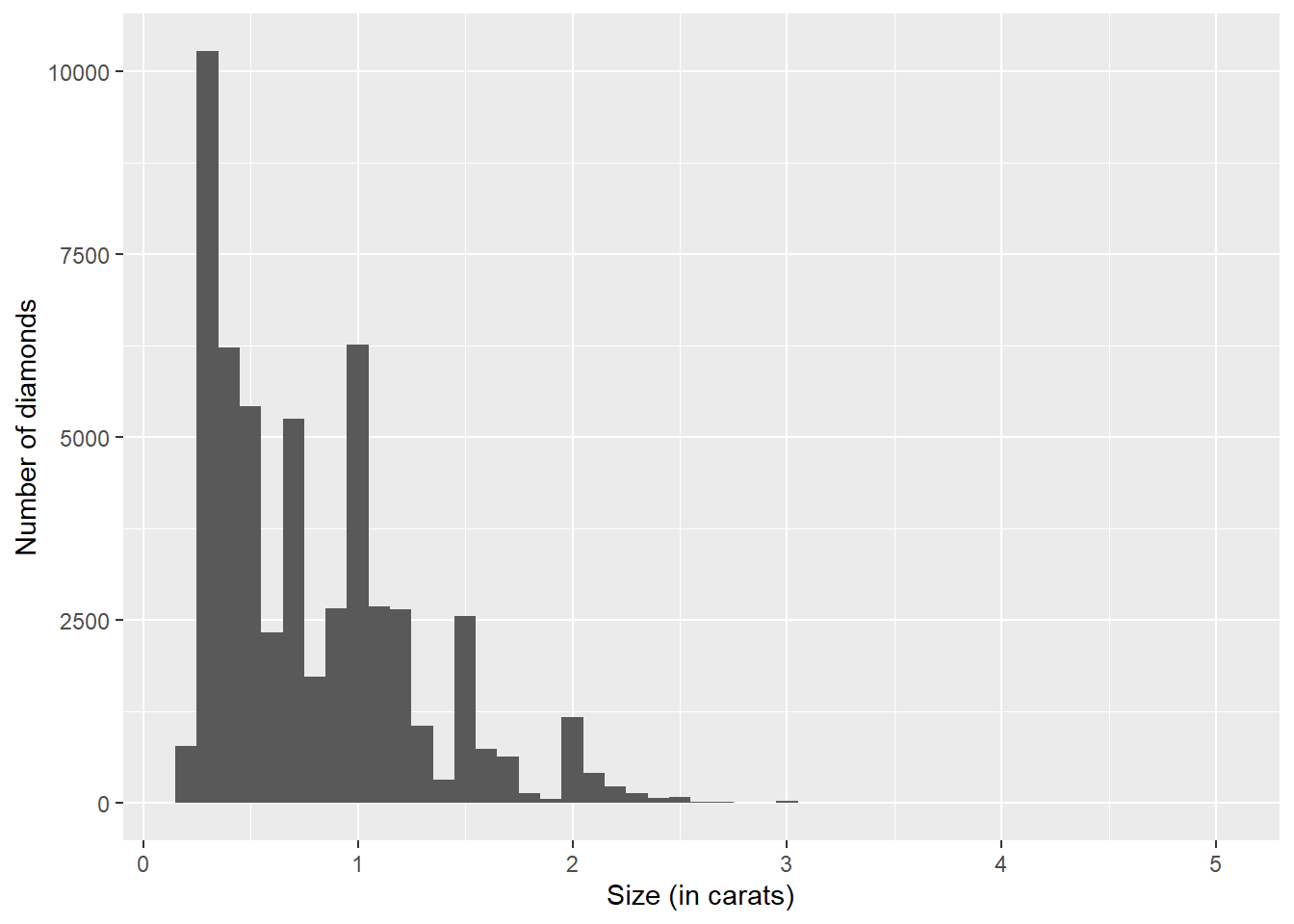

20.2 Call or Run a Function

To call or run the function we type (for example) name(x1, x2). The value of this expression is the value of the expression output. To calculate the value of output the function first copies the value of x1 to argument_1, x2 to argument_2, and so on. The arguments then act as variables within the function. We say that the arguments have been passed to the function. Next the function evaluates the grouped expressions contained in the braces { }; the value of the expression output is returned as the value of the function.

To use the function we first load it (using source or by copying and pasting into R), then call it, supplying suitable arguments.

Example:

rm(list=ls())
source("../scripts/quad3.r")
quad3(1,0,-1)

Note that the name of the function does not have to match the name of the program file, but when a program consists of a single function this is conventional.

20.3 A Function Return

A function always returns a value. For some functions the value returned is unimportant, for example if the function has written its output to a file then there may be no need to return a value as well. In such cases one usually omits the return statement, or returns NULL.

A function may have more than one return statement, in which case it stops after executing the first one it reaches. If there is no return(output) statement then the value returned by the function is the value of the last expression in the braces.

If, when called, the value returned by a function (or any expression) is not assigned to a variable, then it is printed. The expression invisible(x) will return the same value as x, but its value is not printed. For example, some versions of the summary() function use invisible on their returned object.

20.4 Arguments

We think about arguments both when the functions are written and when they are called. The arguments of an existing function can be obtained by calling the formals function.

In order to simplify calling functions, some arguments may be assigned default values, which are used in case the argument is not provided in the call to the function:

Example:

test3 <- function(x = 1) {
  return(x)
  }
test3(2)

[1] 2

test3()

[1] 1

Sometimes you will want to define arguments so that they can take only a small number of different values, and the function will stop informatively if an inappropriate value is passed.

Example:

funk <- function(vibe = c("Do","Be","Dooby","Dooo")) {
  vibe <- match.arg(vibe)
  return(vibe)
  }
funk()

[1] "Do"

funk(Peter)
Error in match.arg(vibe) (from #2) :
'arg' should be one of "Do", "Be", "Dooby", "Dooo"

20.4.1 Argument Matching

R functions arguments can be matched (called) positionally or by name:

Positional matching just means that R assigns the first value to the first argument, the second value to second argument, etc.:

Example:

# Positional match first by argument, default for 'na.rm'
sd(mydata)
# Specify 'x' argument by name, default for 'na.rm'
sd(x = mydata)
# Specify both arguments by name
sd(x = mydata, na.rm = FALSE)

When specifying the function arguments by name, it doesn’t matter in what order you specify them. Named arguments are useful on the command line when you have a long argument list and you want to use the defaults for everything except for an argument near the end of the list:
```
## Specify both arguments by name
sd(na.rm = FALSE, x = mydata)  
```
R also provides partial matching of arguments, where doing so is not ambiguous. This means that argument names in the call to the function do not have to be complete. Reliance on partial matching makes code more fragile.
```
test6 <- function(a = 1, b.c.d = 1) {
  return(a + b.c.d)
  }
test6()
```
```
[1] 2
```
```
test6(b = 5)
```
```
[1] 6
```

20.4.2 The … Argument

...indicates a variable number of arguments that are usually passed on to other functions, it is often used when extending another function and you don’t want to copy the entire argument list of the original function.

The ... argument is necessary when the number of arguments passed to the function cannot be known in advance, e.g. paste(), cat().

Any arguments that appear after ... on the argument list must be named explicitly and cannot be partially matched or matched positionally.

R provides a very useful means of passing arguments, unaltered, from the function that is being called to the functions that are called within it. These arguments do not need to be named explicitly in the outer function, hence providing great flexibility. To use this facility you need to include ... in your argument list. These three dots (an ellipsis) act as a placeholder for any extra arguments given to the function.

Example:

test4 <- function(x, ...) {
  return(sd(x, ...))
  }
test4(1:3)

[1] 1

# Arguments that do not match those in test4 are provided, in order, to any function within test4 that has the dots in the list of arguments to the function call.
test4(c(1:2,NA), na.rm = TRUE)

[1] 0.7071068

Using the dots in this way means that the user has access to all the function arguments without our needing to list them when we define the function.

In general, naming the arguments in the function call is good practice, because it increases the readability and eliminates one potential source of errors.

20.5 Scoping Rules

Arguments and variables that are defined within a function exist only within that function. That is, if you define and use a variable x inside a function, it does not exist outside the function. If variables with the same name exist inside and outside a function, then they are separate and do not interact at all. You can think of a function as a separate environment that communicates with the outside world only through the values of its arguments and its output expression. For example if you execute the command rm(list=ls()) inside a function (which is only rarely a good idea), you only delete those objects that are defined inside the function.

Example:

test <- function(x) {
  y <- x + 1
  return(y)
  }
test(1)

[1] 2

x
Error: Object "x" not found

That part of a program in which a variable is defined is called its scope. Restricting the scope of variables within a function provides an assurance that calling the function will not modify variables outside the function, except by assigning the returned value.

Beware, however, the scope of a variable is not symmetric. That is, variables defined inside a function cannot be seen outside, but variables defined outside the function can be seen inside the function, provided there is not a variable with the same name defined inside.This arrangement makes it possible to write a function whose behavior depends on the context within which it is run.

Example:

test2 <- function(x) {
  y <- x + z
  return(y)
  }
z <- 1
test2(1)

[1] 2

The moral of this example is that it is generally advisable to ensure that the variables you use in a function either are declared as arguments, or have been defined in the function.

20.6 Style

Ideally, the name of your function will be short, but clearly evoke what the function does. Generally, function names should be verbs, and arguments should be nouns. There are some exceptions: nouns are ok if the function computes a very well known noun (i.e. mean() is better than compute_mean()), or accessing some property of an object (i.e. coef() is better than get_coefficients()). Use your best judgement and don’t be afraid to rename a function if you figure out a better name later.

Example:

# Too short
f()

# Not a verb, or descriptive
my_awesome_function()

# Long, but clear
impute_missing()

Additionally, function() should always be followed by squiggly brackets ({}), and the contents should be indented by an additional two spaces. This makes it easier to see the hierarchy in your code by skimming the left-hand margin.

# Missing extra two spaces
density <- function(color, facets, binwidth = 0.1) {
diamonds |> 
  ggplot(aes(x = carat, y = after_stat(density), color = {{ color }})) +
  geom_freqpoly(binwidth = binwidth) +
  facet_wrap(vars({{ facets }}))
}
collapse_years()

# Pipe indented incorrectly
density <- function(color, facets, binwidth = 0.1) {
  diamonds |> 
  ggplot(aes(x = carat, y = after_stat(density), color = {{ color }})) +
  geom_freqpoly(binwidth = binwidth) +
  facet_wrap(vars({{ facets }}))
}